Spatial Phylogenetics Workshop

Joel Nitta

https://joelnitta.com

Assembling Spatial and Genetic Data

Dr. Joel H. Nitta

@joelnitta@fosstodon.org

https://joelnitta.com

• Associate Professor @ Chiba University

• Research interests: Ecology and evolution of ferns

Photo: J-Y Meyer

Basic inputs for spatial phylogenetics

• A phylogeny
  
  
  
  
  
• Spatial occurrence data

… which are linked by taxonomic names (OTUs)

Sources of occurrence data

• Herbaria or museums
• Floras or checklists
• Previous studies
• Your own data

Online sources of occurrence data

• GBIF
• Kew Plants of the World Online (POWO)
• VertNet

etc…

Types of occurrence data

Can take many forms:

• geometric shapes
• points
• checklists
• your own surveys

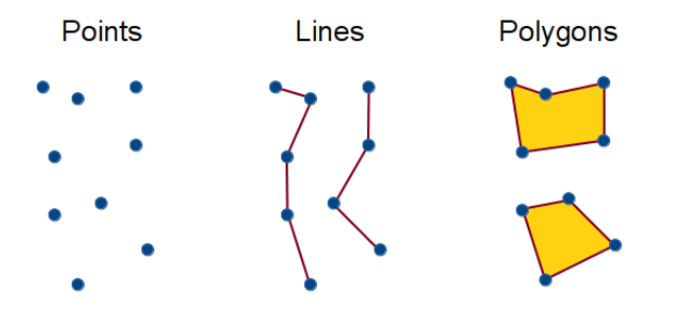
We will focus on point data (the data available from GBIF) during the coding session

GBIF https://www.gbif.org/

GBIF

• GBIF is not one database; it is a portal to many databases

• You should try the web interface first to familiarize yourself with it

• We can’t use the occurrence records in GBIF as-is. They may include many errors (typos, etc.) and need to be checked carefully. More on this during the coding session.

Cleaning occurrence data

• The settings for data cleaning depend on your analysis

• Defaults are a good start, but make sure they make sense!

• For example, if your grid-cell size is 1 degree x 1 degree, you don’t need data to be more exact than that

Coordinate Reference Systems (CRS)

Geographic Coordinate System (GCS)

• Where the data are located
• Round (like the earth)
• Usually in degrees

Projected Coordinate System (PCS)

• How to draw a map of the data
• Flat (like a piece of paper)
• Usually in meters

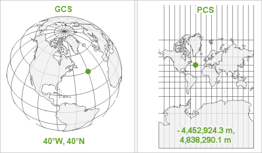
Geographic Coordinate System (GCS)

• Latitude and longitude alone are not enough

• The earth is not a perfect sphere

• GCS defines how to model the earth (e.g., WGS84)

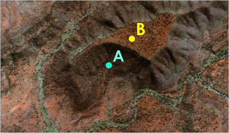
Hiker’s coordinates at 134.577°E, 24.006°S. But where is she (A or B)?

https://www.esri.com/arcgis-blog/products/arcgis-pro/mapping/gcs_vs_pcs/

Projected Coordinate System (PCS)

• The earth is round, but we project it onto flat maps

• The decision of how to do this is not trivial

• There will always be some amount of distortion in area, distance, or direction

https://geoawesomeness.com/wp-content/uploads/2022/03/projections.jpg

Coordinate Reference Systems

• You need to choose an appropriate CRS for your study (there are thousands)

• If you assume that your sampling units have equal area, make sure to use an equal-area projection (e.g., Mollweide)

The Mollweide projection. The orange dots have the same area, but their shape is distorted as you move away from the equator.

https://en.wikipedia.org/wiki/Mollweide_projection

From occurrences to grid-cells

• Raw data are often provided on a per-species basis

• But we are interested in assemblages (grid-cells) of species → need to group species together

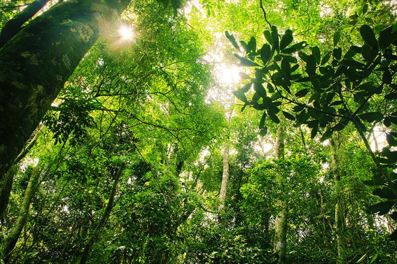
https://phys.org/news/2018-12-local-conditions.html

From occurrences to grid-cells

• For point data, a typical method is to divide the study area into equal size grid-cells, then count the species occurring in each grid-cell

• For shape data, you would overlay the shapes

• For checklist data, the areas may not be equal sized. You could simply use the sampling units in the checklist (e.g., counties, countries, etc.)

Phylogenetic data

• Is there a tree available, or do you need to build it from scratch?

https://images.unsplash.com/

Sources of DNA sequence data

• GenBank
• access in R via the rentrez package
  • (or restez package for larger datasets)

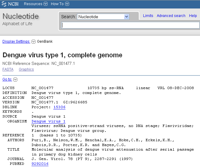
https://a-little-book-of-r-for-bioinformatics.readthedocs.io/

Building a tree from scratch

We don’t have time to cover this today - that is a whole topic of study unto itself!

https://mediacdn.nhbs.com/jackets/jackets_resizer_xlarge/17/170234.jpg

Sources of phylogenetic trees

• Previous publications
• R packages that provide trees (ftolr for ferns)
• Open Tree of Life (rotl R package) (caution!)
• Software that places tips on the tree by taxonomy (caution!)

https://docs.ropensci.org/rotl/logo.svg

What if I don’t have a tree for my group?

• A tree at the species level may not be necessary. Consider doing the analysis at a higher taxonomic level (e.g., genus)

https://www.irasutoya.com/

Is it OK to use taxonomy in place of DNA?

In other words, to place species on the tree based on their taxonomy

• Not such a good idea. This makes a lot of assumptions.
  • Monophyly of the taxa involved
  • Correctness of the taxonomy
• Also produces weird trees with lots of polytomies that may not be suitable for spatial phylogenetics

Taxonomic issues

• Old names
• Misspelled names
• Mismatching synonyms

We need to resolve names to a standard taxonomic database

R tools for assembling spatial and genetic data

Live coding

• Live coding session demonstrating how to use rgbif, CoordinateCleaner, and phyloregion to obtain data

• Code is available here: https://github.com/joelnitta/spatial-phy-workshop/blob/main/tutorials/occ_phy.md

Workflow

A typical workflow involves the following steps:

1. Download occurrence records (rgbif)
2. Clean occurrence records (CoordinateCleaner)
3. Standardize species names (rgbif)
4. Convert points to assemblages (phyloregion)
5. Join assemblage data to phylogeny during spatial phylogenetic analysis (canaper)

What is not covered today

• We don’t have time for demonstrating how to download sequences, assemble them, and conduct phylogenetic analysis (phylogenetic pipelines).

• We will be using a pre-built tree

Other packages: taxonomy

• RTNRS
  • Standardize names using TNRS (Taxonomic Name Resolution Service)
• rWCVP
  • Standardize names to WCVP (World Checklist of Vascular Plants)
• taxadb
  • Standardize names using local databases
• taxastand
  • Standardize names to a custom database

Other packages: occurrences

• occCite
  • Download occurrence data from GBIF and BIEN, and generate references for all databases that contributed
• RBIEN
  • Interface to BIEN database of plant occurrences and traits

Other packages: GenBank data

• rentrez
  • Interface to Entrez databases (including GenBank)
• restez
  • Make a local copy of a portion of GenBank (good for building large trees)

Other packages: phylogenetic pipelines

• phruta
  • Pipeline to download sequences, align them, and build a phylogenetic tree
• phylotaR
  • Pipeline to download and cluster sequences

Other packages: pre-built phylogenies

• ftolr
  • Global fern phylogeny
• fishtree
  • Global fish phylogeny
• rotl
  • R interface to the Open Tree of Life (use with caution)
• U.PhyloMaker
  • Assemble phylogenies by grafting species names onto a backbone (not recommended)

Applications of Spatial Phylogenetics

Spatial phylogenetics can tell us about

• The distribution of endemicity

• Environmental drivers of biodiversity

• Structure of biodiversity

Distribution of endemicity

• Paleoendemism
  • Refugia
  • Colonization by distantly related lineages
• Neoendemism
  • Recent speciation
• Mixed endemism
  • Multiple processes

https://doi.org/10.1073/pnas.1403594111

Distribution of endemicity

• Paleoendemism
  • Refugia
  • Colonization by distantly related lineages
• Neoendemism
  • Recent speciation
• Mixed endemism
  • Multiple processes

https://handwiki.org/wiki/Biology:Neoendemism

Case study: Ferns of Japan

• > 600 species
• Dense sampling
  • 10 x 10 km maps of every species
  • DNA (rbcL) for > 98% of species

Nitta et al. AJB 2022 https://doi.org/10.1002/ajb2.1848

Photos A. Ebihara

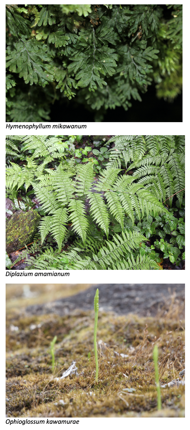
Case study: Ferns of Japan

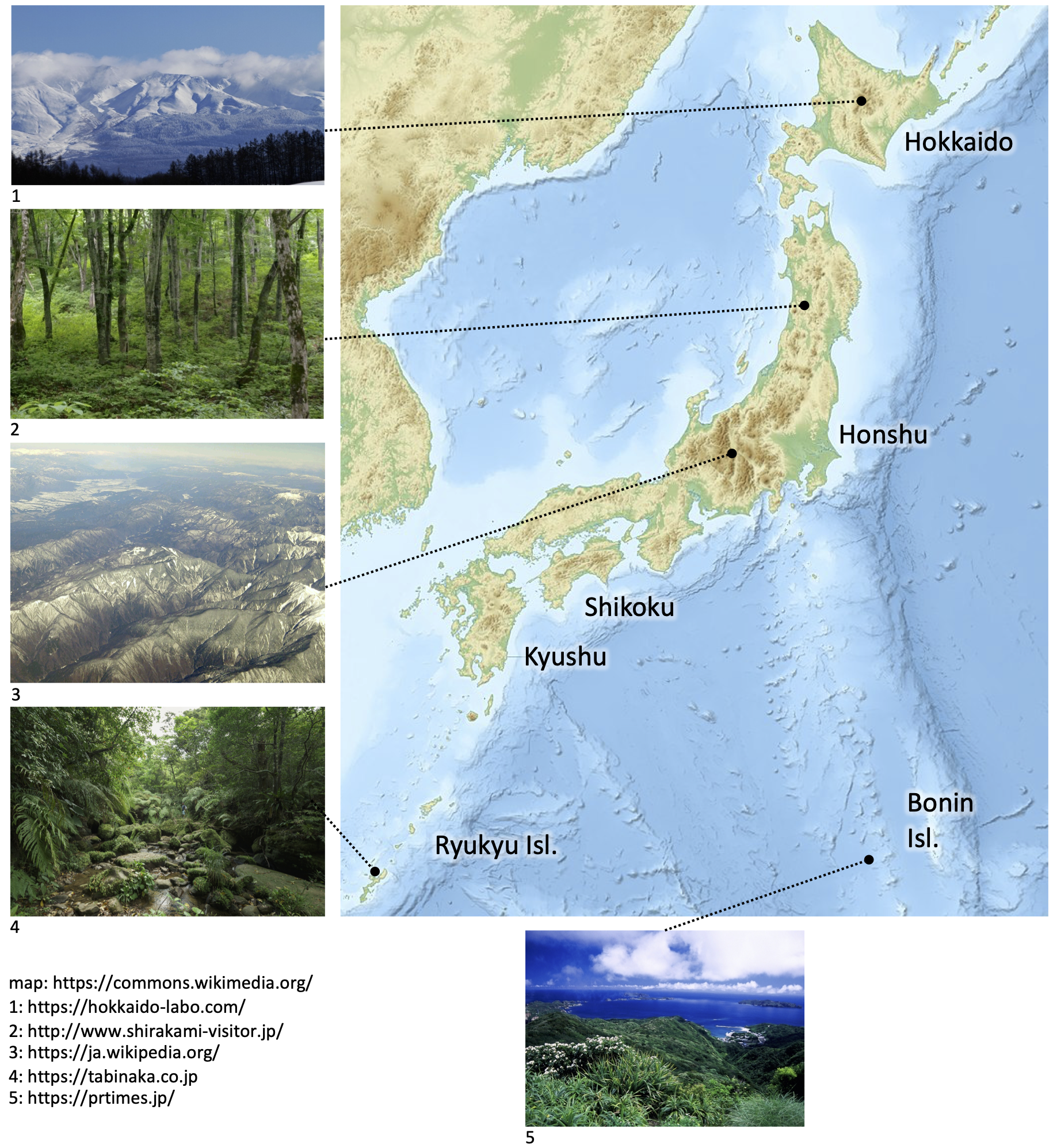
• Variation in climate from N (subarctic) to S (subtropical)

• Variation in elevation

• Main islands continental, southern islands oceanic

Nitta et al. AJB 2022 https://doi.org/10.1002/ajb2.1848

Skewed distribution of endemism

• Southern-most islands are subtropical
  • Very different climate from rest of country
• High rates of mixed- and paleo-endemism
  • Due to distantly related (tropical) lineages

Reproductive mode as driver of biodiversity

Phylogenetic diversity is predicted by % of apogamous (asexual) species

• Apogamous species tend to be hybrids that share identical plastid sequences with other species

Drivers of biodiversity

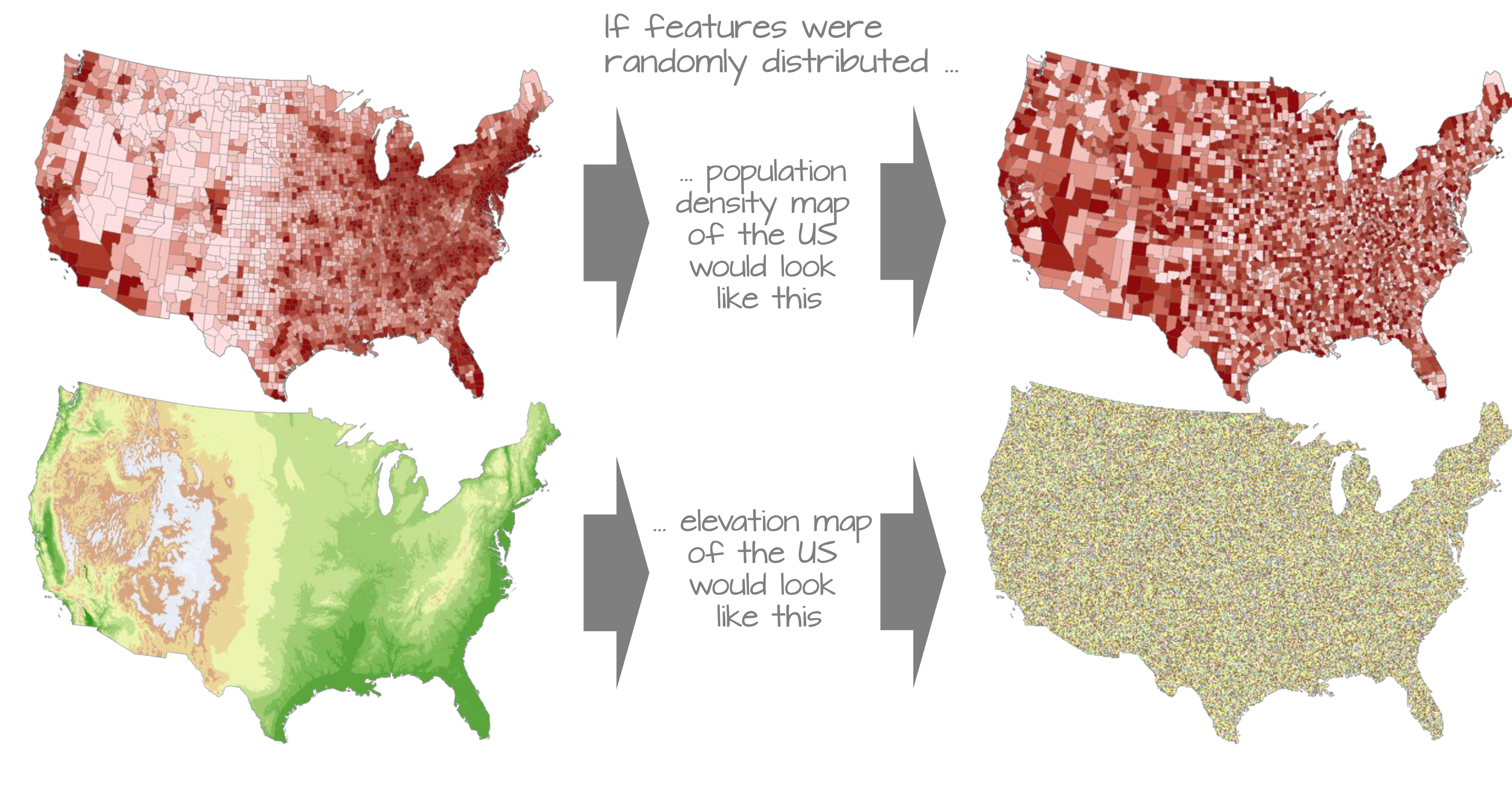
When testing spatial hypotheses (e.g., richness is determined by temperature), we must use spatial methods

Because of spatial autocorrelation

Spatial autocorrelation

https://mgimond.github.io/Spatial/spatial-autocorrelation.html

Accounting for spatial autocorrelation

Compare amount of observed autocorrelation to some expected value: Moran’s I

https://www.cambridge.org/core/books/abs/spatial-analysis-methods-and-practice/spatial-autocorrelation/F6A01B574C69076F28318445C33397E4

Accounting for spatial autocorrelation

Workflow:

• Conduct non-spatial analysis
• Check degree of Moran’s I in model residuals
• If significant, re-do analysis using spatial model

Structure of biodiversity

Understanding the distribution of bio-regions

• Used to be done ad-hoc
  • Not objective
• Newer approaches are quantitative

3-4 regions in ferns of Japan

High rates of endemism on remote islands cause difference in taxonomic and phylogenetic bioregions

Rates of protection vary by biodiversity metric

Spatial phylogenetics in R with canaper

canaper R package

• Can automate CANAPE analysis with R scripts
• Don’t need to switch between Biodiverse and R (do it all in R)

https://docs.ropensci.org/canaper/

Live coding

• Live coding session demonstrating how to use canaper to conduct spatial phylogentic analysis

• Code is available here: https://github.com/joelnitta/spatial-phy-workshop/blob/main/tutorials/canaper.md

Workflow

A typical workflow involves the following steps:

1. Load phylogeny and grid-cell data
2. Determine appropriate null model
3. Conduct randomization test
4. Categorize results
5. Plot results

Survey

Please fill out the post-workshop survey:

https://forms.gle/Dh1TdJctskWXVHSW7