R for Reproducible Scientific Analysis: All in One View

Content from RとRStudio入門

Last updated on 2025-07-01 | Edit this page

Estimated time: 55 minutes

Overview

Questions

RStudio内でどのように操作するのか？
Rとの対話方法は？
環境をどのように管理するのか？
パッケージをどのようにインストールするのか？

Objectives

RStudioの各ペインの目的と使用方法を説明する
RStudio内のボタンやオプションの場所を見つける
変数を定義する
データを変数に代入する
インタラクティブなRセッションでワークスペースを管理する
数学および比較演算子を使用する
関数を呼び出す
パッケージを管理する

ワークショップを始める前に

ワークショップで使用する一部のパッケージが正しくインストールされない（または全くインストールされない）場合があるため、お使いのマシンにRとRStudioの最新バージョンがインストールされていることを確認してください。

なぜRとRStudioを使うのか？

Software CarpentryワークショップのRセクションへようこそ！

科学は多段階のプロセスです。実験を設計してデータを収集した後、本当の楽しみは分析から始まります！このレッスンでは、R言語の基本を教えるとともに、科学プロジェクトのためのコードを整理するベストプラクティスを学び、作業をより簡単にする方法を紹介します。

データを分析するためにMicrosoft ExcelやGoogleスプレッドシートを使用することもできますが、これらのツールは柔軟性やアクセス性に限界があります。さらに、元データの変更や探索の手順を共有することが難しいため、これは「再現可能な」研究にとって重要なポイントです（再現可能な研究についてはこちら）。

したがって、このレッスンでは、RとRStudioを使用してデータの探索を始める方法を学びます。RプログラムはWindows、Mac、Linuxオペレーティングシステムで利用可能で、上記のリンクから無料でダウンロードできます。Rを実行するために必要なのはRプログラムだけです。

しかし、Rをより使いやすくするために、同じくダウンロードしたRStudioというプログラムを使用します。RStudioは無料でオープンソースの統合開発環境（IDE）で、組み込みエディタを提供し、すべてのプラットフォームで動作します（サーバー上でも利用可能）。バージョン管理やプロジェクト管理との統合など、多くの利点があります。

概要

生データから始め、探索的な分析を行い、結果をグラフでプロットする方法を学びます。この例では、gapminder.orgのデータセットを使用し、時間を通じた各国の人口情報を扱います。データをRに読み込むことができますか？セネガルの人口をプロットできますか？アジア大陸の国々の平均所得を計算できますか？このレッスンの終わりまでに、これらの国々の人口を1分以内にプロットできるようになります！

基本レイアウト

RStudioを初めて開くと、次の3つのパネルが表示されます：

インタラクティブなRコンソール/ターミナル（左全体）
環境/履歴/接続（右上のタブ）
ファイル/プロット/パッケージ/ヘルプ/ビューア（右下のタブ）

ファイル（例えばRスクリプト）を開くと、上部左にエディタパネルも表示されます。

Rスクリプト

Rコンソールに書いたコマンドはファイルに保存し、再実行することができます。このようなRコードを含むファイルをRスクリプトと呼びます。Rスクリプトは名前の末尾が.Rとなっており、それがRスクリプトであることを示します。

RStudio内でのワークフロー

RStudio内で作業する主な方法は2つあります：

インタラクティブなRコンソール内でテストや試行を行い、そのコードをコピーして.Rファイルに貼り付け、後で実行する。
- 小規模なテストや初期の段階では効果的です。
- しかし、すぐに手間がかかるようになります。
最初から.Rファイルに記述し、RStudioのショートカットキーを使用して「Run」コマンドを実行し、現在の行、選択した行、または変更した行をインタラクティブなRコンソールに送る。
- これは作業を始める良い方法です。すべてのコードが後で使用するために保存されます。
- RStudio内またはRのsource()関数を使用して作成したファイルを実行できます。

ヒント：コードのセグメントを実行する

RStudioでは、エディタウィンドウからコードを実行する柔軟性があります。ボタン、メニューオプション、およびキーボードショートカットがあります。現在の行を実行するには、次の方法があります：

エディタパネルの上部にある「Run」ボタンをクリックする
「Code」メニューから「Run Lines」を選択する
WindowsまたはLinuxではCtrl+Return、OS Xでは⌘+Returnを押す（このショートカットはボタンの上にマウスをホバーさせると確認できます）。コードブロックを実行するには、選択して「Run」をクリックします。最近実行したコードブロックを修正した場合、セクションを再選択して「Run」を押す必要はありません。次のボタン「Re-run the previous region」を使用すると、修正を含む前のコードブロックを実行できます。

R入門

Rでの作業の多くは、インタラクティブなRコンソール内で行います。ここでは、すべてのコードを実行し、Rスクリプトファイルに追加する前にアイデアを試すのに便利な環境です。RStudioのコンソールは、コマンドライン環境でRと入力した場合と同じです。

Rのインタラクティブセッションを開くと、最初に情報が表示され、その後に「>」と点滅するカーソルが現れます。これは、シェルレッスンで学んだシェル環境と多くの点で似ています。「Read, evaluate, print loop」（読み取り、評価、印刷ループ）の考え方に基づいて動作します：コマンドを入力すると、Rがそれを実行し、結果を返します。

Rを計算機として使う

Rで最も簡単なことは、算術を行うことです：

R

1 + 100

OUTPUT

[1] 101

Rは答えを表示し、その前に”[1]“を付けます。[1]はコンソールに表示される行の最初の要素のインデックスを示します。ベクトルのインデックスについての詳細は、エピソード6：データのサブセット化を参照してください。

不完全なコマンドを入力すると、R

は完了を待機します。Unix Shellのbashに慣れている場合、この動作をbashで見たことがあるかもしれません。

R

> 1 +

OUTPUT

「>」ではなく「+」が表示された場合、Rはコマンドの完了を待機しています。コマンドをキャンセルしたい場合はEscを押すと、RStudioは「>」プロンプトに戻ります。

ヒント：コマンドのキャンセル

コマンドラインからRを使用している場合は、RStudioの代わりにEscではなくCtrl+Cを使用してコマンドをキャンセルする必要があります。これはMacユーザーにも適用されます！

コマンドのキャンセルは、不完全なコマンドを終了させるだけでなく、予想以上に時間がかかる場合にコードの実行を停止したり、現在書いているコードを削除したりするためにも役立ちます。

Rを計算機として使用する場合、演算の順序は学校で学んだものと同じです。

優先順位が高いものから低いものへ：

括弧：(, )
累乗：^または**
乗算：*
除算：/
加算：+
減算：-

R

3 + 5 * 2

OUTPUT

[1] 13

評価の順序を変更したい場合や意図を明確にしたい場合は、括弧を使用してグループ化します。

R

(3 + 5) * 2

OUTPUT

[1] 16

必要ない場合は煩雑になりますが、意図を明確にできます。他の人が後でコードを読むかもしれないことを忘れないでください。

R

(3 + (5 * (2 ^ 2))) # 読みにくい
3 + 5 * 2 ^ 2       # 規則を覚えていれば明快
3 + 5 * (2 ^ 2)     # 規則を忘れた場合はこれが助けになる

各コード行の後にあるテキストは「コメント」と呼ばれます。ハッシュ記号#の後に続く内容は、コードを実行する際にRによって無視されます。

非常に小さいまたは大きい数値は、科学表記法で表示されます：

R

2/10000

OUTPUT

[1] 2e-04

これは「10^XXで掛ける」という短縮形です。したがって、2e-4は2 * 10^(-4)の短縮形です。

科学表記法で数値を書くこともできます：

R

5e3  # マイナスがない点に注意

OUTPUT

[1] 5000

数学関数

Rには多くの組み込み数学関数があります。関数を呼び出すには、関数名を入力し、その後に開き括弧と閉じ括弧を続けます。関数は引数を入力として受け取ります。関数の括弧内に入力したものはすべて引数と見なされます。関数によって引数の数は異なり、引数を必要としないものから複数の引数を必要とするものまであります。例：

R

getwd() # 絶対パスを返す

この例では引数は不要ですが、以下の数学関数では結果を計算するために値を渡す必要があります。

R

sin(1)  # 三角関数

OUTPUT

[1] 0.841471

R

log(1)  # 自然対数

OUTPUT

[1] 0

R

log10(10) # 常用対数（底10）

OUTPUT

[1] 1

R

exp(0.5) # e^(1/2)

OUTPUT

[1] 1.648721

Rのすべての関数を覚えようとする必要はありません。Googleで検索するか、関数名の最初の数文字を覚えていれば、RStudioのタブ補完機能を使うことができます。

RStudioの大きな利点の一つは、オートコンプリート機能があることです。これにより、関数、引数、および受け取る値を簡単に調べることができます。

コマンド名の前に?を付けると、そのコマンドのヘルプページが開きます。RStudioを使用している場合、’Help’ペインに表示されます。ターミナルでRを使用している場合は、ブラウザでヘルプページが開きます。ヘルプページにはコマンドの詳細な説明と動作の仕組みが含まれています。ページの下部までスクロールすると、通常、コマンドの使用例が掲載されています。後ほど例を見ていきます。

比較演算

Rでは比較を行うこともできます：

R

1 == 1  # 等しい（等号が2つ、"等しい"と読む）

OUTPUT

[1] TRUE

R

1 != 2  # 等しくない（"等しくない"と読む）

OUTPUT

[1] TRUE

R

1 < 2  # より小さい

OUTPUT

[1] TRUE

R

1 <= 1  # 以下

OUTPUT

[1] TRUE

R

1 > 0  # より大きい

OUTPUT

[1] TRUE

R

1 >= -9 # 以上

OUTPUT

[1] TRUE

ヒント：数値の比較

数値を比較する際の注意点として、整数（小数を含まない数値型）以外を比較する場合は、==を使用しないでください。

コンピュータは小数を特定の精度でしか表現できないため、Rが表示する際に同じに見える2つの数値が、内部表現では異なる場合があります。このわずかな差異は「数値計算誤差（Machine numeric tolerance）」と呼ばれます。

代わりにall.equal関数を使用してください。

さらに詳しく知りたい方はこちら：http://floating-point-gui.de/

変数と代入

代入演算子<-を使用して、値を変数に格納できます：

R

x <- 1/40

代入は値を表示しません。代わりに、それを後で使用するために変数というものに格納します。この場合、xには値0.025が格納されています：

R

OUTPUT

[1] 0.025

正確には、この格納された値は浮動小数点数と呼ばれる分数の10進数近似値です。

RStudioの右上ペインにあるEnvironmentタブを確認すると、xとその値が表示されていることがわかります。変数xは、数値を期待する計算の中で数値の代わりに使用できます：

R

log(x)

OUTPUT

[1] -3.688879

また、変数には再代入も可能です：

R

x <- 100

以前はxに0.025が格納されていましたが、現在は100が格納されています。

代入値には、代入先の変数を含めることもできます：

R

x <- x + 1 # RStudioの右上タブでxの説明が更新されることに注目
y <- x * 2

代入の右辺には有効なR式を使用できます。右辺は代入が行われる前に完全に評価されます。

変数名には、文字、数字、アンダースコア、ピリオドを含めることができますが、スペースは含められません。また、変数名は文字またはピリオドで始める必要があります（数字やアンダースコアでは始めることはできません）。ピリオドで始まる変数は隠し変数と見なされます。

長い変数名については、異なる人が異なる規約を使用します。その例として：

periods.between.words
underscores_between_words
camelCaseToSeparateWords

どれを使用するかは自由ですが、一貫性を保つことが重要です。

代入には=演算子を使用することも可能です：

R

x = 1/40

しかし、これはRユーザーの間ではあまり一般的ではありません。最も重要なのは、使用する演算子に一貫性を持つことです。<-を使用したほうが混乱が少ない場合もあり、コミュニティでは最も一般的に使われています。そのため、<-を使用することを推奨します。

チャレンジ 1

次の中で有効なRの変数名はどれですか？

R

min_height
max.height
_age
.mass
MaxLength
min-length
2widths
celsius2kelvin

チャレンジ1の解答

次のものはR変数として使用できます：

R

min_height
max.height
MaxLength
celsius2kelvin

次のものは隠し変数を作成します：

R

.mass

次のものは変数を作成できません：

R

_age
min-length
2widths

ベクトル化

Rの特徴の1つに、Rがベクトル化されているという点があります。つまり、変数や関数にベクトルを値として持たせることができます。物理学や数学におけるベクトルとは異なり、Rにおけるベクトルは同じデータ型の値が順序付けられた集合を指します。例：

R

1:5

OUTPUT

[1] 1 2 3 4 5

R

2^(1:5)

OUTPUT

[1]  2  4  8 16 32

R

x <- 1:5
2^x

OUTPUT

[1]  2  4  8 16 32

この機能は非常に強力で、今後のレッスンでさらに詳しく説明します。

環境の管理

Rセッションとやり取りするための便利なコマンドがいくつかあります。

lsを使用すると、グローバル環境（現在のRセッション）に保存されているすべての変数と関数を一覧表示できます：

R

ls()

OUTPUT

[1] "x" "y"

ヒント：隠しオブジェクト

シェルと同様に、lsではデフォルトで”.”で始まる変数や関数は表示されません。すべてのオブジェクトを一覧表示するには、ls(all.names=TRUE)と入力してください。

ここでは、lsに引数を渡していませんが、関数を呼び出すために括弧は必要です。

lsだけを入力すると、オブジェクト一覧ではなくコードが表示されます：

R

ls

OUTPUT

function (name, pos = -1L, envir = as.environment(pos), all.names = FALSE,
    pattern, sorted = TRUE)
{
    if (!missing(name)) {
        pos <- tryCatch(name, error = function(e) e)
        if (inherits(pos, "error")) {
            name <- substitute(name)
            if (!is.character(name))
                name <- deparse(name)
            warning(gettextf("%s converted to character string",
                sQuote(name)), domain = NA)
            pos <- name
        }
    }
    all.names <- .Internal(ls(envir, all.names, sorted))
    if (!missing(pattern)) {
        if ((ll <- length(grep("[", pattern, fixed = TRUE))) &&
            ll != length(grep("]", pattern, fixed = TRUE))) {
            if (pattern == "[") {
                pattern <- "\\["
                warning("replaced regular expression pattern '[' by  '\\\\['")
            }
            else if (length(grep("[^\\\\]\\[<-", pattern))) {
                pattern <- sub("\\[<-", "\\\\\\[<-", pattern)
                warning("replaced '[<-' by '\\\\[<-' in regular expression pattern")
            }
        }
        grep(pattern, all.names, value = TRUE)
    }
    else all.names
}
<bytecode: 0x555f519a3fc0>
<environment: namespace:base>

これはどういうことでしょうか？

Rではすべてがオブジェクトであり、オブジェクト名だけを入力すると、その内容が表示されます。先ほど作成したオブジェクトxには1, 2, 3, 4, 5が格納されています：

R

OUTPUT

[1] 1 2 3 4 5

オブジェクトlsには、ls関数を動作させるRコードが格納されています！関数の仕組みや作成方法については後のレッスンで説明します。

不要になったオブジェクトを削除するには、rmを使用します：

R

rm(x)

多くのオブジェクトが環境にあり、それらをすべて削除したい場合は、lsの結果をrm関数に渡します：

R

rm(list = ls())

この場合、2つの関数を組み合わせています。演算の順序と同様に、最も内側の括弧内の内容が最初に評価されます。

この場合、lsの結果がrmのlist引数として使用されるよう指定しています。引数に値を名前で割り当てる場合、必ず=演算子を使用する必要があります！

代わりに<-を使用すると、予期しない副作用が発生するか、エラーメッセージが表示される可能性があります：

R

rm(list <- ls())

ERROR

Error in rm(list <- ls()): ... must contain names or character strings

ヒント：警告とエラー

Rが予期しない動作をした場合は注意してください！エラーはRが計算を続行できない場合に発生します。一方、警告は通常、関数が実行されたものの、期待通りに動作しなかったことを意味します。

どちらの場合も、Rが表示するメッセージには問題を解決するための手がかりが含まれていることが多いです。

Rパッケージ

Rにはパッケージを作成することで関数を追加することができます。また、他の人が作成したパッケージを利用することも可能です。この執筆時点で、CRAN（Comprehensive R Archive Network）には10,000を超えるパッケージが利用可能です。RとRStudioにはパッケージを管理するための機能があります：

インストールされているパッケージを確認するには、installed.packages()を入力します。
パッケージをインストールするには、install.packages("packagename")と入力します。ここでpackagenameはパッケージ名で、引用符で囲みます。
インストール済みのパッケージを更新するには、update.packages()を入力します。
パッケージを削除するには、remove.packages("packagename")を使用します。
パッケージを利用可能にするには、library(packagename)を入力します。

RStudioの右下ペインの「Packages」タブからもパッケージを表示、ロード、デタッチすることができます。このタブをクリックすると、インストール済みのパッケージがチェックボックス付きで表示されます。パッケージ名の横にあるチェックボックスがオンの場合、そのパッケージはロードされており、オフの場合はロードされていません。空のボックスをクリックするとそのパッケージがロードされ、チェックボックスをクリックするとパッケージがデタッチされます。

また、「Packages」タブの上部にある「Install」ボタンと「Update」ボタンを使用して、パッケージをインストールおよび更新できます。

チャレンジ 2

次のプログラムの各文の後で、各変数の値はどうなるでしょうか？

R

mass <- 47.5
age <- 122
mass <- mass * 2.3
age <- age - 20

チャレンジ2の解答

R

mass <- 47.5

この時点で変数massの値は47.5になります。

R

age <- 122

この時点で変数ageの値は122になります。

R

mass <- mass * 2.3

既存の値47.5に2.3を掛け、新しい値109.25をmassに格納します。

R

age <- age - 20

既存の値122から20を引き、新しい値102をageに格納します。

チャレンジ 3

前のチャレンジのコードを実行し、massとageを比較するコマンドを書きなさい。massはageより大きいですか？

チャレンジ3の解答

この質問に答える方法の1つとして、次のように>を使用できます：

R

mass > age

OUTPUT

[1] TRUE

このコードは、109.25が102より大きいため、論理値TRUEを返すはずです。

チャレンジ 4

作業環境を整理し、massとageの変数を削除しなさい。

チャレンジ4の解答

このタスクを達成するには、rmコマンドを使用します：

R

rm(age, mass)

チャレンジ 5

以下のパッケージをインストールしなさい：ggplot2, plyr, gapminder

チャレンジ5の解答

必要なパッケージをインストールするには、install.packages()コマンドを使用します。

R

install.packages("ggplot2")
install.packages("plyr")
install.packages("gapminder")

1つのinstall.packages()コマンドで複数のパッケージ

をインストールする別の方法は次のとおりです：

R

install.packages(c("ggplot2", "plyr", "gapminder"))

Instructor Note

ggplot2をインストールする際、一部のユーザーは依存関係フラグを使用する必要がある場合があります。これは既知のバグではなく、ワークショップの実施中に確認されたエラーを解決するための推奨事項です：

R

install.packages("ggplot2", dependencies = TRUE)

Key Points

RStudioを使用してRプログラムを作成および実行します。
Rには通常の算術演算子と数学関数があります。
<-を使用して変数に値を代入します。
ls()を使用してプログラム内の変数を一覧表示します。
rm()を使用してプログラム内のオブジェクトを削除します。
install.packages()を使用してパッケージ（ライブラリ）をインストールします。

Content from RStudio を使ったプロジェクト管理

Last updated on 2025-07-01 | Edit this page

Estimated time: 30 minutes

Overview

Questions

R でプロジェクトをどのように管理できますか？

Objectives

RStudio で自己完結型のプロジェクトを作成する

はじめに

科学的なプロセスは本質的に段階的なものであり、多くのプロジェクトはランダムなメモ、一部のコード、次に原稿と進行し、最終的にはすべてが混ざり合ってしまうことがよくあります。

プロジェクトを再現可能な方法で管理することは、科学を再現可能にするだけでなく、生活をより簡単にします。
— Vince Buffalo (@vsbuffalo) 2013年4月15日

ほとんどの人はプロジェクトを次のように整理しがちです：

このような方法を絶対に避けるべき理由は数多くあります：

データのどのバージョンがオリジナルで、どれが修正済みなのかを区別するのが非常に難しい。
様々な拡張子のファイルが混在して、非常に散らかる。
必要なものを見つけたり、正確なコードで生成した正しい図表を関連付けたりするのに非常に時間がかかる。

良いプロジェクト構成は、最終的に生活をより簡単にします：

データの整合性を確保しやすくなる。
他の人（研究室の同僚、共同研究者、指導教員）とコードを共有するのが簡単になる。
原稿の投稿時にコードを簡単にアップロードできる。
しばらく休んだ後にプロジェクトを再開しやすくなる。

考えられる解決策

幸いなことに、作業を効果的に管理するためのツールやパッケージが存在します。

RStudio の最も強力で便利な機能の一つがプロジェクト管理機能です。本日はこれを使って自己完結型の再現可能なプロジェクトを作成します。

チャレンジ 1: 自己完結型プロジェクトの作成

RStudio で新しいプロジェクトを作成します：

「File」メニューをクリックし、「New Project」を選択します。
「New Directory」をクリックします。
「New Project」をクリックします。
プロジェクトを保存するディレクトリの名前（例：my_project）を入力します。
「Create a git repository」のチェックボックスが表示される場合は選択します。
「Create Project」ボタンをクリックします。

作成した RStudio プロジェクトを開く最も簡単な方法は、ファイルシステムをたどって保存したディレクトリに移動し、.Rproj ファイルをダブルクリックすることです。これにより RStudio が開き、R セッションが .Rproj ファイルと同じディレクトリで開始します。データ、プロット、スクリプトはすべてプロジェクトディレクトリに関連付けられます。さらに、RStudio プロジェクトは複数のプロジェクトを同時に開くことが可能で、それぞれのプロジェクトディレクトリに分離されます。これにより、複数のプロジェクトを開いても相互に干渉しません。

チャレンジ 2: ファイルシステムを使った RStudio プロジェクトの開き方

RStudio を終了します。
チャレンジ 1 で作成したプロジェクトのディレクトリに移動します。
そのディレクトリ内の .Rproj ファイルをダブルクリックします。

プロジェクト管理のベストプラクティス

プロジェクトを整理するための「ベスト」な方法はありませんが、管理を容易にするために従うべきいくつかの一般原則があります：

データを読み取り専用として扱う

プロジェクトを設定する際の最も重要な目標はこれです。データの収集は通常、時間と費用がかかります。データをインタラクティブに操作する（例：Excel で）と、データの出所や収集後にどのように変更されたかを把握できなくなります。そのため、データを「読み取り専用」として扱うのが良い考えです。

データのクリーニング

多くの場合、データは「汚れて」おり、R（または他のプログラミング言語）で有用な形式にするために大幅な前処理が必要です。このタスクは「データマンジング」と呼ばれることもあります。これらのスクリプトを別のフォルダに保存し、クリーンなデータセットを保持する「読み取り専用」データフォルダを作成することで、両者の混同を防ぐことができます。

生成された出力を使い捨てとみなす

スクリプトによって生成されたものはすべて使い捨てとみなすべきです：スクリプトからすべてを再生成できる必要があります。

出力を管理する方法はたくさんあります。各分析ごとに異なるサブディレクトリを持つ出力フォルダを用意すると、後で便利です。多くの分析は探索的で最終プロジェクトに使用されないことが多く、一部の分析はプロジェクト間で共有されることもあります。

ヒント: 科学的コンピューティングのための「十分に良い」実践

科学的コンピューティングのための「十分に良い」実践では、プロジェクトの構成について以下の推奨事項を挙げています：

各プロジェクトを専用のディレクトリに配置し、そのディレクトリにプロジェクト名を付ける。
プロジェクトに関連するテキスト文書を doc ディレクトリに配置する。
生データとメタデータを data ディレクトリに、クリーンアップや分析中に生成されたファイルを results ディレクトリに配置する。
プロジェクトのスクリプトやプログラムのソースを src ディレクトリに配置し、他から持ち込んだプログラムやローカルでコンパイルしたプログラムを bin ディレクトリに配置する。
すべてのファイルに内容や機能を反映した名前を付ける。

関数の定義と適用を分離する

R を効率的に使用する最も効果的な方法の一つは、最初に .R スクリプトに実行したいコードを書き、RStudio のキーボードショートカットを使用するか「Run」ボタンをクリックして、選択した行をインタラクティブな R コンソールで実行することです。

プロジェクトの初期段階では、最初の .R スクリプトファイルに多くの直接実行されるコード行が含まれることがよくあります。プロジェクトが進むにつれて、再利用可能なコードチャンクが独自の関数に分離されます。これらの関数を保存するためのフォルダと分析スクリプトを保存するためのフォルダを分けるのが良いアイデアです。

データを data ディレクトリに保存する

良好なディレクト

リ構造ができたら、データファイルを data/ ディレクトリに保存します。

チャレンジ 3

このリンクから CSV ファイルをダウンロードしてください。

ファイルをダウンロードします（上記リンクを右クリック -> 「リンク先を名前を付けて保存」/「名前を付けて保存」、またはリンクをクリックしページが読み込まれた後に Ctrl+S を押すか、メニューの「ファイル」 -> 「ページを名前を付けて保存」を選択）。
gapminder_data.csv という名前で保存されていることを確認します。
ファイルをプロジェクト内の data/ フォルダに保存します。

後ほどこのデータを読み込み、確認します。

チャレンジ 4

R に読み込む前に、コマンドラインからデータセットについての一般的な情報を得ることは有益です。これにより、R に読み込む際の判断に役立ちます。コマンドラインシェルを使用して以下の質問に答えてください：

ファイルのサイズはどれくらいですか？
このファイルには何行のデータがありますか？
このファイルにはどのような値が含まれていますか？

チャレンジ 4 の解答

次のコマンドをシェルで実行します：

SH

ls -lh data/gapminder_data.csv

OUTPUT

-rw-r--r-- 1 runner docker 80K Jul  1 00:26 data/gapminder_data.csv

ファイルサイズは 80K です。

SH

wc -l data/gapminder_data.csv

OUTPUT

1705 data/gapminder_data.csv

行数は 1705 行です。データの内容は次のようになります：

SH

head data/gapminder_data.csv

OUTPUT

country,year,pop,continent,lifeExp,gdpPercap
Afghanistan,1952,8425333,Asia,28.801,779.4453145
Afghanistan,1957,9240934,Asia,30.332,820.8530296
Afghanistan,1962,10267083,Asia,31.997,853.10071
Afghanistan,1967,11537966,Asia,34.02,836.1971382
Afghanistan,1972,13079460,Asia,36.088,739.9811058
Afghanistan,1977,14880372,Asia,38.438,786.11336
Afghanistan,1982,12881816,Asia,39.854,978.0114388
Afghanistan,1987,13867957,Asia,40.822,852.3959448
Afghanistan,1992,16317921,Asia,41.674,649.3413952

ヒント: RStudio のコマンドライン

RStudio のコンソールペインにある「Terminal」タブを使用すると、RStudio 内で直接コマンドラインを操作できます。

作業ディレクトリ

R の現在の作業ディレクトリを知ることは重要です。なぜなら、他のファイルにアクセスする必要があるとき（例：データファイルをインポートする場合）、R は現在の作業ディレクトリを基準にそれらのファイルを探すからです。

新しい RStudio プロジェクトを作成するたびに、そのプロジェクトの新しいディレクトリが作成されます。既存の .Rproj ファイルを開くと、そのプロジェクトが開き、R の作業ディレクトリがそのファイルがあるフォルダに設定されます。

チャレンジ 5

getwd() コマンドを使用するか、RStudio のメニューを使って現在の作業ディレクトリを確認します。

コンソールで getwd()（“wd” は “working directory” の略）と入力し、Enter を押します。
ファイルペインで、data フォルダをダブルクリックして開く（または他の任意のフォルダに移動）。作業ディレクトリに戻るには、ファイルペインの「More」をクリックし、「Go To Working Directory」を選択します。

setwd() コマンドを使用するか、RStudio のメニューを使って作業ディレクトリを変更します。

コンソールで setwd("data") と入力し、Enter を押します。その後、getwd() と入力して Enter を押し、新しい作業ディレクトリを確認します。
RStudio ウィンドウ上部のメニューで「Session」をクリックし、「Set Working Directory」を選択して「Choose Directory」をクリックします。その後、開いたウィンドウでプロジェクトディレクトリに戻り、「Open」をクリックします。コンソールに setwd コマンドが自動的に表示されます。

ヒント: ファイルが存在しないエラー

R コードでファイルを参照しようとして「ファイルが存在しない」というエラーが出た場合は、作業ディレクトリを確認するのが良いです。ファイルへの絶対パスを指定するか、作業ディレクトリ内（またはそのサブフォルダ）にファイルを保存し、相対パスを指定する必要があります。

バージョン管理

プロジェクトではバージョン管理を使用することが重要です。RStudio で Git を使用する方法についての良いレッスンはこちらを参照してください。

Key Points

RStudio を使用して一貫したレイアウトでプロジェクトを作成および管理する。
生データを読み取り専用として扱う。
生成された出力を使い捨てとみなす。
関数の定義と適用を分離する。

Content from ヘルプの利用

Last updated on 2025-07-01 | Edit this page

Estimated time: 20 minutes

Overview

Questions

R でどのようにしてヘルプを得ることができますか？

Objectives

関数や特殊な演算子に関する R のヘルプファイルを読むことができる。
問題を解決するためのパッケージを特定するために CRAN タスクビューを利用できる。
仲間に助けを求める方法を理解する。

ヘルプファイルを読む

R および各パッケージには関数用のヘルプファイルが用意されています。特定のパッケージに含まれる関数についてヘルプを検索する際の一般的な構文は次の通りです：

R

?function_name
help(function_name)

たとえば、write.table() のヘルプファイルを見てみましょう。この関数に似た機能を持つ関数を今後のエピソードで使用します。

R

?write.table()

これにより、RStudio ではヘルプページが表示され、R 本体ではプレーンテキストとして表示されます。

各ヘルプページは次のようなセクションに分かれています：

Description（説明）: 関数が何をするかの詳細な説明。
Usage（使用法）: 関数の引数とそのデフォルト値（変更可能）。
Arguments（引数）: 各引数が期待するデータの説明。
Details（詳細）: 注意すべき重要な点。
Value（戻り値）: 関数が返すデータ。
See Also（関連項目）: 有用な関連関数。
Examples（例）: 関数の使用例。

関数によってはセクションが異なる場合がありますが、これらが主なポイントです。

関連する関数が同じヘルプファイルを参照する場合があることに注意してください：

R

?write.table()
?write.csv()

これらの関数は非常に似た用途を持ち、引数も共通しているため、パッケージ作者が同じヘルプファイルで文書化していることがよくあります。

ヒント: 実例を実行する

ヘルプページ内の Examples セクションからコードをハイライトして Ctrl+Return を押すと、RStudio コンソールで実行されます。関数の動作を素早く理解する方法です。

ヒント: ヘルプファイルを読む

R の大きな課題の一つは、利用可能な関数の数が膨大であることです。すべての関数の正しい使用法を記憶するのは現実的ではありません。しかし、ヘルプファイルを利用すれば、記憶する必要はありません！

特殊な演算子

特殊な演算子に関するヘルプを検索するには、引用符またはバッククォートを使用します：

R

?"<-"
?`<-`

パッケージに関するヘルプ

多くのパッケージには「ビネット」と呼ばれるチュートリアルや拡張的な例のドキュメントが含まれています。引数なしで vignette() を実行すると、インストール済みのすべてのパッケージのビネットが表示されます。特定のパッケージについては vignette(package="パッケージ名") を使用します。特定のビネットを開くには vignette("ビネット名") を実行します。

パッケージにビネットがない場合は、通常、次のコマンドでヘルプを探せます：

R

help("パッケージ名")

また、RStudio には多くのパッケージ向けに優れたチートシートがあります。

関数名の一部を覚えている場合

関数がどのパッケージに属しているか、または正確なスペルがわからない場合、ファジー検索が可能です：

R

??function_name

ファジー検索では文字列の近似一致を検索します。たとえば、作業ディレクトリを設定する関数に「set」が含まれていることを覚えている場合、次のように検索できます：

R

??set

どこから始めるべきかわからない場合

どの関数やパッケージを使用すべきかわからない場合、 CRAN Task Views を利用するとよいでしょう。これは、パッケージを分野別にグループ化した特別なリストで、出発点として適しています。

コードが動作しない場合: 仲間に助けを求める

関数の使用に問題がある場合、その答えのほとんどはすでに Stack Overflow で回答されています。 [r] タグを使って検索してください。質問の仕方については、Stack Overflow の良い質問の仕方のページを参照してください。

答えが見つからない場合、以下の便利な関数を使って仲間に助けを求めるとよいでしょう：

R

?dput

この関数は、使用しているデータを他の人が自分の R セッションでコピー＆ペーストできる形式に出力します。

R

sessionInfo()

OUTPUT

R version 4.5.1 (2025-06-13)
Platform: x86_64-pc-linux-gnu
Running under: Ubuntu 22.04.5 LTS

Matrix products: default
BLAS:   /usr/lib/x86_64-linux-gnu/blas/libblas.so.3.10.0
LAPACK: /usr/lib/x86_64-linux-gnu/lapack/liblapack.so.3.10.0  LAPACK version 3.10.0

locale:
 [1] LC_CTYPE=C.UTF-8       LC_NUMERIC=C           LC_TIME=C.UTF-8
 [4] LC_COLLATE=C.UTF-8     LC_MONETARY=C.UTF-8    LC_MESSAGES=C.UTF-8
 [7] LC_PAPER=C.UTF-8       LC_NAME=C              LC_ADDRESS=C
[10] LC_TELEPHONE=C         LC_MEASUREMENT=C.UTF-8 LC_IDENTIFICATION=C

time zone: UTC
tzcode source: system (glibc)

attached base packages:
[1] stats     graphics  grDevices utils     datasets  methods   base

loaded via a namespace (and not attached):
[1] compiler_4.5.1 tools_4.5.1    yaml_2.3.10    knitr_1.48     xfun_0.49
[6] renv_1.1.4     evaluate_1.0.1

この関数は、R の現在のバージョンやロードしているパッケージを表示します。これは他の人が問題を再現し、デバッグするのに役立ちます。

チャレンジ 1

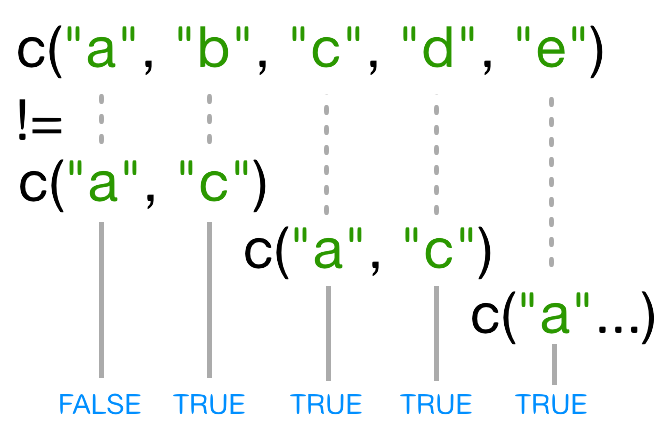
c 関数のヘルプページを見てください。次のコードを評価した場合、どのようなベクトルが作成されると思いますか？

R

c(1, 2, 3)
c('d', 'e', 'f')
c(1, 2, 'f')

チャレンジ 1 の解答

c() 関数はすべての要素が同じ型のベクトルを作成します。最初の場合、要素は数値型、 2 番目の場合は文字型、そして 3 番目の場合も文字型です。数値型の値は文字型に「強制変換」されます。

チャレンジ 2

paste 関数のヘルプを見てください。この関数を後ほど使用します。 sep 引数と collapse 引数の違いは何ですか？

チャレンジ 2 の解答

paste() 関数のヘルプを見るには以下を実行します：

R

help("paste")
?paste

sep と collapse の違いは少し複雑です。paste 関数は任意の数の引数を受け取り、それぞれが任意の長さのベクトルであることができます。 sep 引数は連結される各項目の間に使用される文字列を指定します（デフォルトはスペース）。結果は、paste に渡された最も長い引数と同じ長さのベクトルです。一方、collapse 引数は、連結後の要素を指定された区切り文字を使用して「まとめて結合」することを示します。その結果、単一の文字列になります。

引数を明示的に指定することが重要です。たとえば sep = "," と入力すると、関数は区切り文字として “,” を使用し、結合する項目としてではないと認識します。

例：

R

paste(c("a","b"), "c")

OUTPUT

[1] "a c" "b c"

R

paste(c("a","b"), "c", ",")

OUTPUT

[1] "a c ," "b c ,"

R

paste(c("a","b"), "c", sep = ",")

OUTPUT

[1] "a,c" "b,c"

R

paste(c("a","b"), "c", collapse = "|")

OUTPUT

[1] "a c|b c"

R

paste(c("a","b"), "c", sep = ",", collapse = "|")

OUTPUT

[1] "a,c|b,c"

（詳細については、?paste ヘルプページの末尾の例を参照するか、example('paste') を試してください。）

チャレンジ 3

ヘルプを使用して、タブ区切り（\t）の列と小数点が “.”（ピリオド）で表される表形式のファイルを読み込むために使用できる関数（および関連するパラメータ）を見つけてください。特に国際的な同僚と協力している場合、小数点の表記（例：コンマ対ピリオド）は異なる場合があるため、この確認が重要です。ヒント：??"read table" を使用して表形式データの読み込みに関連する関数を調べてください。

チャレンジ 3 の解答

タブ区切りファイルを小数点がピリオドで表される形式で読み込む標準的な R 関数は read.delim() です。また、read.table(file, sep="\t") を使用することもできます（read.table() のデフォルトの小数点はピリオドです）。ただし、データファイルにハッシュ（#）文字が含まれている場合は、comment.char 引数を変更する必要があるかもしれません。

その他のリソース

Key Points

R のオンラインヘルプを取得するには help() を使用します。

Content from データ構造

Last updated on 2025-07-01 | Edit this page

Estimated time: 55 minutes

Overview

Questions

R でデータをどのように読み取ることができますか？
R の基本的なデータ型は何ですか？
R でカテゴリ情報をどのように表現しますか？

Objectives

5 つの主なデータ型を特定できるようになる。
データフレームを探索し始め、ベクトルやリストとの関連を理解する。
R からオブジェクトの型、クラス、構造に関する質問ができるようになる。
“names”、“class”、“dim” 属性の情報を理解する。

R の最も強力な機能の 1 つは、スプレッドシートや CSV ファイルにすでに保存されているような表形式データを処理する能力です。まずは、data/ ディレクトリに feline-data.csv という名前の小さなデータセットを作成しましょう：

R

cats <- data.frame(coat = c("calico", "black", "tabby"),
                    weight = c(2.1, 5.0, 3.2),
                    likes_catnip = c(1, 0, 1))

次に、cats を CSV ファイルとして保存します。引数名を明示的に指定することは良い習慣であり、関数が変更されたデフォルト値を認識できます。この場合は row.names = FALSE を設定しています。引数名やそのデフォルト値を確認するには、?write.csv を使用してヘルプファイルを表示してください。

R

write.csv(x = cats, file = "data/feline-data.csv", row.names = FALSE)

新しいファイル feline-data.csv の内容は次の通りです：

R

coat,weight,likes_catnip
calico,2.1,1
black,5.0,0
tabby,3.2,1

ヒント: R でテキストファイルを編集する

または、テキストエディタ（Nano）や RStudio の File -> New File -> Text File メニュー項目を使用して data/feline-data.csv を作成することもできます。

このデータを R に読み込むには、以下のコマンドを使用します：

R

cats <- read.csv(file = "data/feline-data.csv")
cats

OUTPUT

    coat weight likes_catnip
1 calico    2.1            1
2  black    5.0            0
3  tabby    3.2            1

read.table 関数は、CSV ファイル（csv = comma-separated values）などのテキストファイルに保存された表形式データを読み取るために使用されます。タブやカンマは、CSV ファイルでデータポイントを区切るために最も一般的に使用される記号です。R では read.table の便利なバージョンとして read.csv（データがカンマで区切られている場合）と read.delim（データがタブで区切られている場合）が用意されています。この 3 つの中で、read.csv が最も一般的に使用されます。必要に応じて、デフォルトの区切り記号を変更することもできます。

データが因子かどうかを確認する

最近、R がテキストデータを処理する方法が変更されました。以前は、R はテキストデータを自動的に “因子” という形式に変換していましたが、現在は “文字列” という形式で処理されるようになりました。因子の使用用途については後ほど学びますが、ほとんどの場合は必要なく、使用することで複雑になるだけです。そのため、新しい R バージョンではテキストデータが “文字列” として読み取られます。因子が自動的に作成されているかを確認し、必要に応じて文字列形式に変換してください：

入力データの型を確認するには、str(cats) を入力します。
出力で、コロンの後にある 3 文字のコードを確認します：num と chr のみが表示される場合は、レッスンを続けることができます。このボックスはスキップしてください。fct が見つかった場合は、次の手順に進んでください。
R が因子データを自動的に作成しないようにするには、以下のコードを実行します：options(stringsAsFactors = FALSE)。その後、cats テーブルを再読み込みして変更を反映させます。
R を再起動するたびに、このオプションを設定する必要があります。忘れないように、データを読み込む前にスクリプトの最初の行のいずれかに含めてください。
R バージョン 4.0.0 以降では、テキストデータは因子に変換されなくなりました。問題を回避するためにこのバージョン以降をインストールすることを検討してください。研究所や会社のコンピュータを使用している場合は、管理者に依頼してください。

データセットをすぐに探索し始めることができます。たとえば、$ 演算子を使用して列を指定します：

R

cats$weight

OUTPUT

[1] 2.1 5.0 3.2

R

cats$coat

OUTPUT

[1] "calico" "black"  "tabby"

列に対して操作を実行することもできます：

R

## たとえば、スケールが 2kg 軽いことが判明した場合：
cats$weight + 2

OUTPUT

[1] 4.1 7.0 5.2

R

paste("My cat is", cats$coat)

OUTPUT

[1] "My cat is calico" "My cat is black"  "My cat is tabby"

しかし、次のコードではどうでしょうか？

R

cats$weight + cats$coat

ERROR

Error in cats$weight + cats$coat: non-numeric argument to binary operator

ここで何が起こったのかを理解することが、R でデータを成功裏に分析する鍵です。

データ型

最後のコマンドがエラーを返す理由が 2.1 と "black" を加算するのは無意味だからだと推測したなら、あなたは正しいです！これはプログラミングにおける重要な概念である データ型 に関する直感をすでに持っているということです。データの型を調べるには、次のように入力します：

R

typeof(cats$weight)

OUTPUT

[1] "double"

主なデータ型は次の 5 種類です：double、integer、complex、logical、character。歴史的な理由で、double は numeric とも呼ばれます。

R

typeof(3.14)

OUTPUT

[1] "double"

R

typeof(1L) # L サフィックスを付けると数値を整数に強制します（R はデフォルトで浮動小数点数を使用）

OUTPUT

[1] "integer"

R

typeof(1+1i)

OUTPUT

[1] "complex"

R

typeof(TRUE)

OUTPUT

[1] "logical"

R

typeof('banana')

OUTPUT

[1] "character"

分析がどれだけ複雑であっても、R ではすべてのデータがこれらの基本的なデータ型のいずれかとして解釈されます。この厳格さには非常に重要な意味があります。

別の猫の詳細を追加した情報が、ファイル data/feline-data_v2.csv に保存されています。

R

file.show("data/feline-data_v2.csv")

R

coat,weight,likes_catnip
calico,2.1,1
black,5.0,0
tabby,3.2,1
tabby,2.3 or 2.4,1

この新しい猫データを以前と同じ方法で読み込み、weight 列にどのようなデータ型が含まれているか確認します：

R

cats <- read.csv(file="data/feline-data_v2.csv")
typeof(cats

$weight)

OUTPUT

[1] "character"

あらら、weight 列の型が double ではなくなっています！以前と同じ計算を試みると、問題が発生します：

R

cats$weight + 2

ERROR

Error in cats$weight + 2: non-numeric argument to binary operator

何が起こったのでしょうか？私たちが扱っている cats データは データフレーム と呼ばれるものです。データフレームは、R で最も一般的で多用途な データ構造 の 1 つです。データフレームの特定の列には異なるデータ型を混在させることはできません。この場合、R はデータフレーム列 weight のすべてを double として読み取らなかったため、列全体のデータ型がその列内のすべてに適した型に変わります。

R が CSV ファイルを読み取ると、それは データフレーム として読み込まれます。そのため、cats CSV ファイルを読み込むと、データフレームとして保存されます。データフレームは str() 関数によって表示される最初の行で認識できます：

R

str(cats)

OUTPUT

'data.frame':	4 obs. of  3 variables:
 $ coat        : chr  "calico" "black" "tabby" "tabby"
 $ weight      : chr  "2.1" "5" "3.2" "2.3 or 2.4"
 $ likes_string: int  1 0 1 1

データフレーム は行と列で構成され、各列は同じ数の行を持ちます。データフレームの異なる列は異なるデータ型で構成できます（これがデータフレームを非常に柔軟にする理由です）が、特定の列内ではすべてが同じ型である必要があります（例：ベクトル、因子、リストなど）。

この振る舞いをさらに調査する間、猫のデータから余分な行を削除し、それを再読み込みしましょう：

feline-data.csv:

coat,weight,likes_catnip
calico,2.1,1
black,5.0,0
tabby,3.2,1

そして RStudio 内で：

R

cats <- read.csv(file="data/feline-data.csv")

ベクトルと型の強制変換

この挙動をよりよく理解するために、別のデータ構造である ベクトル を紹介します。

R

my_vector <- vector(length = 3)
my_vector

OUTPUT

[1] FALSE FALSE FALSE

R におけるベクトルは、基本的に順序付けられた要素のリストです。ただし、特別な条件として、ベクトル内のすべての要素は同じ基本データ型である必要があります。データ型を指定しない場合、デフォルトで logical 型になります。また、任意の型の空のベクトルを宣言することも可能です。

R

another_vector <- vector(mode='character', length=3)
another_vector

OUTPUT

[1] "" "" ""

あるオブジェクトがベクトルかどうかを確認することもできます：

R

str(another_vector)

OUTPUT

 chr [1:3] "" "" ""

このコマンドのやや難解な出力は、このベクトルに含まれる基本データ型（この場合は chr、文字型）を示し、ベクトル内の要素数（この場合は [1:3]）、および実際に含まれる要素（この場合は空の文字列）を示します。同様に次のコマンドを実行すると、

R

str(cats$weight)

OUTPUT

 num [1:3] 2.1 5 3.2

cats$weight もベクトルであることがわかります。R のデータフレームに読み込まれる列はすべてベクトルです。これが、R が列内のすべての要素を同じ基本データ型に強制する理由の根本です。

討論 1

なぜ R は列に含まれるデータに対してこれほど厳格なのでしょうか？この厳格さは私たちにどのように役立つのでしょうか？

討論 1 の解答

列内のすべてのデータが同じであることで、データに対して単純な仮定を行うことができます。たとえば、列の 1 つの要素を数値として解釈できるなら、列内のすべての要素を数値として解釈できます。そのため、毎回確認する必要がなくなります。この一貫性こそが、人々が「クリーンデータ」と呼ぶものです。長い目で見ると、この厳格な一貫性は R におけるデータ操作を非常に簡単にしてくれます。

ベクトルを結合する際の型の強制変換

明示的な内容を持つベクトルを c() 関数で作成できます：

R

combine_vector <- c(2,6,3)
combine_vector

OUTPUT

[1] 2 6 3

これまで学んだ内容を考えると、次のコードは何を生成すると思いますか？

R

quiz_vector <- c(2,6,'3')

これは 型の強制変換 と呼ばれるもので、予想外の結果をもたらすことがあり、基本データ型と R がそれをどのように解釈するかを理解する必要があります。R は、異なる型（ここでは double と character）が単一のベクトルに結合される場合、それらをすべて同じ型に強制します。例を見てみましょう：

R

coercion_vector <- c('a', TRUE)
coercion_vector

OUTPUT

[1] "a"    "TRUE"

R

another_coercion_vector <- c(0, TRUE)
another_coercion_vector

OUTPUT

[1] 0 1

型の階層

型の強制変換ルールは次の通りです：
logical -> integer -> double (“numeric”) -> complex -> character
この矢印は「変換される」と読めます。たとえば、logical と character を結合すると、結果は character に変換されます：

R

c('a', TRUE)

OUTPUT

[1] "a"    "TRUE"

character ベクトルは、印刷時にクォートで囲まれていることで簡単に認識できます。

逆方向の強制変換を試みる場合は、as. 関数を使用します：

R

character_vector_example <- c('0','2','4')
character_vector_example

OUTPUT

[1] "0" "2" "4"

R

character_coerced_to_double <- as.double(character_vector_example)
character_coerced_to_double

OUTPUT

[1] 0 2 4

R

double_coerced_to_logical <- as.logical(character_coerced_to_double)
double_coerced_to_logical

OUTPUT

[1] FALSE  TRUE  TRUE

R が基本データ型を他の型に強制する際に驚くべきことが起こる場合があります！型の強制変換の細かい点はさておき、重要なのは：データが予想していた形式と異なる場合、それは型の強制変換が原因である可能性が高いです。ベクトルやデータフレームの列内のすべてのデータが同じ型であることを確認してください。さもなければ、予想外の問題が発生する可能性があります！

しかし、強制変換は非常に便利な場合もあります！たとえば、cats データの likes_catnip 列は数値型ですが、実際には 1 と 0 がそれぞれ TRUE と FALSE を表しています。このデータには logical 型を使用すべきです。この型は TRUE または FALSE の 2 状態を持ち、データの意味に完全に一致します。この列を logical に「強制変換」するには、as.logical 関数を使用します：

R

cats$likes_catnip

OUTPUT

[1] 1 0 1

R

cats$likes_catnip <- as.logical(cats$likes_catnip)
cats$likes_catnip

OUTPUT

[1]  TRUE FALSE  TRUE

チャレンジ 1

データ分析の重要な部分は、入力データのクリーンアップです。入力データがすべて同じ形式（例：数値）であることを知っていると、分析がはるかに簡単になります！型の強制変換に関する章で扱った猫のデータセットをクリーンアップしましょう。

コードテンプレートをコピー

RStudio で新しいスクリプトを作成し、以下のコードをコピー＆ペーストしてください。その後、以下のタスクを参考にギャップ（______）を埋めてください。

# データを読み込み
cats <- read.csv("data/feline-data_v2.csv")

# 1. データを表示
_____

# 2. 表の概要をデータ型と共に表示
_____(cats)

# 3. "weight" 列の現在のデータ型 __________。
#    正しいデータ型は： ____________。

# 4. 4 番目の "weight" データポイントを指定された 2 つの値の平均に修正
cats$weight[4] <- 2.35
#    効果を確認するためにデータを再表示
cats

# 5. "weight" を正しいデータ型に変換
cats$weight <- ______________(cats$weight)

#    自分でテストするために平均を計算
mean(cats$weight)

# 正しい平均値（NA ではない）が表示されたら、演習は完了です！

タスクの手順

1. データを表示する

最初のステートメント（read.csv(...)）を実行します。その後、データをコンソールに表示します。

ヒント 1.1

任意の変数の内容を表示するには、その名前を入力します。

チャレンジ 1.1 の解答

2 つの正しい解答：

R

cats

OUTPUT

    coat weight likes_catnip
1 calico    2.1         TRUE
2  black    5.0        FALSE
3  tabby    3.2         TRUE

R

print(cats)

OUTPUT

    coat weight likes_catnip
1 calico    2.1         TRUE
2  black    5.0        FALSE
3  tabby    3.2         TRUE

2. データ型の概要を表示する

データ型はデータ自体と同じくらい重要です。以前見た関数を使用して、cats テーブルのすべての列のデータ型を表示します。

ヒント 1.2

「データ型」の章で、データ型を表示する 2 つの関数を見ました。1 つはデータ型の名前だけを出力し、もう 1 つは短い形式のデータ型と最初の値を出力しました。ここでは後者を使用します。

チャレンジ 1.2 の解答

R

str(cats)

OUTPUT

'data.frame':	3 obs. of  3 variables:
 $ coat        : chr  "calico" "black" "tabby"
 $ weight      : num  2.1 5 3.2
 $ likes_catnip: logi  TRUE FALSE TRUE

3. 必要

なデータ型はどれですか？

表示されるデータ型は、このデータ（猫の体重）には適していません。必要なデータ型はどれですか？

なぜ read.csv() 関数は正しいデータ型を選ばなかったのでしょうか？
コメントのギャップに猫の体重に適したデータ型を埋めてください！

ヒント 1.3

型の階層のセクションに戻り、利用可能なデータ型を確認してください。

チャレンジ 1.3 の解答

体重は連続スケール（実数）で表されます。この場合の R のデータ型は “double”（“numeric” とも呼ばれます）です。
4 行目の値は “2.3 or 2.4” であり、数値ではなく英単語が含まれています。そのため、“character” 型が選ばれます。同じ列内のすべての値が同じデータ型である必要があるため、列全体がテキスト型になっています。

4. 問題のある値を修正する

問題のある 4 行目に新しい体重値を割り当てるコードが提供されています。実行する前に考えてみてください。この例のように数値を割り当てた後のデータ型はどうなりますか？実行後にデータ型を確認して、自分の予測が正しいか確認してください。

ヒント 1.4

2 つの異なるデータ型が組み合わされた場合の型の階層を再確認してください。

チャレンジ 1.4 の解答

列 “weight” のデータ型は “character” です。割り当てるデータ型は “double” です。異なるデータ型を組み合わせると、次の階層でより高いデータ型に変換されます：

logical < integer < double < complex < character

したがって、列はまだ “character” 型です！これを “double” 型に手動で変換する必要があります。

5. 列 “weight” を正しいデータ型に変換する

猫の体重は数値です。しかし、列にはまだ適切なデータ型が設定されていません。この列を浮動小数点数に強制変換してください。

ヒント 1.5

データ型を変換する関数は as. で始まります。このスクリプトの上部で関数を確認するか、RStudio のオートコンプリート機能を使用してください。 “as.” と入力し、TAB キーを押します。

チャレンジ 1.5 の解答

歴史的な理由で、2 つの同義の関数があります：

R

cats$weight <- as.double(cats$weight)
cats$weight <- as.numeric(cats$weight)

基本的なベクトル関数

c() 関数を使用すると、既存のベクトルに新しい要素を追加することができます：

R

ab_vector <- c('a', 'b')
ab_vector

OUTPUT

[1] "a" "b"

R

combine_example <- c(ab_vector, 'SWC')
combine_example

OUTPUT

[1] "a"   "b"   "SWC"

また、数列を生成することも可能です：

R

mySeries <- 1:10
mySeries

OUTPUT

 [1]  1  2  3  4  5  6  7  8  9 10

R

seq(10)

OUTPUT

 [1]  1  2  3  4  5  6  7  8  9 10

R

seq(1, 10, by=0.1)

OUTPUT

 [1]  1.0  1.1  1.2  1.3  1.4  1.5  1.6  1.7  1.8  1.9  2.0  2.1  2.2  2.3  2.4
[16]  2.5  2.6  2.7  2.8  2.9  3.0  3.1  3.2  3.3  3.4  3.5  3.6  3.7  3.8  3.9
[31]  4.0  4.1  4.2  4.3  4.4  4.5  4.6  4.7  4.8  4.9  5.0  5.1  5.2  5.3  5.4
[46]  5.5  5.6  5.7  5.8  5.9  6.0  6.1  6.2  6.3  6.4  6.5  6.6  6.7  6.8  6.9
[61]  7.0  7.1  7.2  7.3  7.4  7.5  7.6  7.7  7.8  7.9  8.0  8.1  8.2  8.3  8.4
[76]  8.5  8.6  8.7  8.8  8.9  9.0  9.1  9.2  9.3  9.4  9.5  9.6  9.7  9.8  9.9
[91] 10.0

ベクトルについていくつかの質問をすることもできます：

R

sequence_example <- 20:25
head(sequence_example, n=2)

OUTPUT

[1] 20 21

R

tail(sequence_example, n=4)

OUTPUT

[1] 22 23 24 25

R

length(sequence_example)

OUTPUT

[1] 6

R

typeof(sequence_example)

OUTPUT

[1] "integer"

ベクトルの特定の要素を取得するには、角括弧記法を使用します：

R

first_element <- sequence_example[1]
first_element

OUTPUT

[1] 20

特定の要素を変更するには、角括弧を矢印の右側に使用します：

R

sequence_example[1] <- 30
sequence_example

OUTPUT

[1] 30 21 22 23 24 25

チャレンジ 2

1 から 26 までの数を含むベクトルを作成します。その後、このベクトルを 2 倍にします。

チャレンジ 2 の解答

R

x <- 1:26
x <- x * 2

次に紹介するデータ構造は list です。リストは他のデータ型よりもシンプルで、何でも入れることができるのが特徴です。ベクトルでは要素の基本データ型を統一する必要がありましたが、リストは異なるデータ型を持つことができます：

R

list_example <- list(1, "a", TRUE, 1+4i)
list_example

OUTPUT

[[1]]
[1] 1

[[2]]
[1] "a"

[[3]]
[1] TRUE

[[4]]
[1] 1+4i

str() を使用してオブジェクトの構造を表示すると、すべての要素のデータ型を確認できます：

R

str(list_example)

OUTPUT

List of 4
 $ : num 1
 $ : chr "a"
 $ : logi TRUE
 $ : cplx 1+4i

リストの用途は何でしょうか？例えば、異なるデータ型を持つ関連データを整理できます。これは、Excel のスプレッドシートのように複数の表をまとめるのと似ています。他にも多くの用途があります。

次の章で、驚くかもしれない別の例を紹介します。

リストの特定の要素を取得するには 二重角括弧 を使用します：

R

list_example[[2]]

OUTPUT

[1] "a"

リストの要素には名前を付けることもできます。名前を値の前に等号で指定します：

R

another_list <- list(title = "Numbers", numbers = 1:10, data = TRUE )
another_list

OUTPUT

$title
[1] "Numbers"

$numbers
 [1]  1  2  3  4  5  6  7  8  9 10

$data
[1] TRUE

これにより 名前付きリスト が生成されます。これで新しいアクセス方法が追加されます！

R

another_list$title

OUTPUT

[1] "Numbers"

名前

名前を使用すると、要素に意味を持たせることができます。これにより、データだけでなく説明情報も持つことができます。これはオブジェクトに貼り付けられるラベルのような メタデータ です。R ではこれは属性と呼ばれます。属性により、オブジェクトをさらに操作することが可能になります。ここでは、定義された名前で要素にアクセスすることができます。

名前を使用してベクトルやリストにアクセスする

名前付きリストの生成方法はすでに学びました。名前付きベクトルを生成する方法も非常に似ています。以前このような関数を見たことがあるはずです：

R

pizza_price <- c( pizzasubito = 5.64, pizzafresh = 6.60, callapizza = 4.50 )

しかし、要素の取得方法はリストとは異なります：

R

pizza_price["pizzasubito"]

OUTPUT

pizzasubito
       5.64

リストのアプローチは機能しません：

R

pizza_price$pizzafresh

ERROR

Error in pizza_price$pizzafresh: $ operator is invalid for atomic vectors

このエラーメッセージを覚えておくと役立ちます。同じようなエラーに遭遇することが多いですが、これはリストと勘違いしてベクトルの要素にアクセスしようとした場合に発生します。

名前の取得と変更

名前だけに興味がある場合は、names() 関数を使用します：

R

names(pizza_price)

OUTPUT

[1] "pizzasubito" "pizzafresh"  "callapizza"

ベクトルの要素にアクセスしたり変更したりする方法を学びました。同じことが名前についても可能です：

R

names(pizza_price)[3]

OUTPUT

[1] "callapizza"

R

names(pizza_price)[3] <- "call-a-pizza"
pizza_price

OUTPUT

 pizzasubito   pizzafresh call-a-pizza
        5.64         6.60         4.50

チャレンジ 3

pizza_price の名前のデータ型は何ですか？str() または typeof() 関数を使用して調べてください。

チャレンジ 3 の解答

オブジェクトの名前を取得するには、その名前を names(...) で囲みます。同様に、名前のデータ型を取得するには、全体をさらに typeof(...) で囲みます：

typeof(names(pizza))

または、コードをわかりやすくするために新しい変数を使用します：

n <- names(pizza)
typeof(n)

チャレンジ 4

既存のベクトルやリストの一部の名前を変更する代わりに、オブジェクトのすべての名前を設定することも可能です。次のコード形式を使用します（すべての大文字部分を置き換えてください）：

names( OBJECT ) <-  CHARACTER_VECTOR

アルファベットの各文字に番号を割り当てるベクトルを作成しましょう！

1 から 26 の数列を持つ letter_no というベクトルを作成します。
R には LETTERS という組み込みオブジェクトがあります。これは A から Z までの 26 文字を含むベクトルです。この 26 文字を letter_no の名前として設定します。
letter_no["B"] を呼び出して、値が 2 であることを確認してください！

チャレンジ 4 の解答

letter_no <- 1:26   # or seq(1,26)
names(letter_no) <- LETTERS
letter_no["B"]

データフレーム

このレッスンの冒頭でデータフレームについて簡単に触れましたが、それはデータの表形式を表しています。例として示した猫のデータフレームについては詳細に掘り下げていませんでした：

R

cats

OUTPUT

    coat weight likes_catnip
1 calico    2.1         TRUE
2  black    5.0        FALSE
3  tabby    3.2         TRUE

ここで少し驚くべきことに気づくかもしれません。次のコマンドを実行してみましょう：

R

typeof(cats)

OUTPUT

[1] "list"

データフレームが「内部的にはリストのように見える」ことがわかります。以前、リストについて次のように説明しました：

リストは異なる型のデータを整理するためのもの

データフレームの列は、それぞれが異なる型のベクトルであり、同じ表に属することで整理されています。

データフレームは実際にはベクトルのリストです。データフレームが特別なのは、すべてのベクトルが同じ長さでなければならない点です。

この「特別さ」はどのようにオブジェクトに組み込まれているのでしょうか？R がそれを単なるリストではなく、表として扱うのはなぜでしょう？

R

class(cats)

OUTPUT

[1] "data.frame"

クラス は名前と同様に、オブジェクトに付加される属性です。この属性は、そのオブジェクトが人間にとって何を意味するのかを示します。

ここで疑問に思うかもしれません：なぜオブジェクトの型を判断するための関数がもう一つ必要なのでしょうか？すでに typeof() がありますよね？
typeof() はオブジェクトがコンピュータ内でどのように構築されているかを教えてくれます。一方、class() はオブジェクトの人間にとっての意味を示します。したがって、typeof() の出力は R で固定されています（主に 5 種類のデータ型）が、class() の出力は R パッケージによって多様で拡張可能です。

cats の例では、整数型、倍精度数値型、論理型の変数が含まれています。すでに見たように、データフレームの各列はベクトルです：

R

cats$coat

OUTPUT

[1] "calico" "black"  "tabby"

R

cats[,1]

OUTPUT

[1] "calico" "black"  "tabby"

R

typeof(cats[,1])

OUTPUT

[1] "character"

R

str(cats[,1])

OUTPUT

 chr [1:3] "calico" "black" "tabby"

一方、各行は異なる変数の観測値であり、それ自体がデータフレームであり、異なる型の要素で構成されることができます：

R

cats[1,]

OUTPUT

    coat weight likes_catnip
1 calico    2.1         TRUE

R

typeof(cats[1,])

OUTPUT

[1] "list"

R

str(cats[1,])

OUTPUT

'data.frame':	1 obs. of  3 variables:
 $ coat        : chr "calico"
 $ weight      : num 2.1
 $ likes_catnip: logi TRUE

チャレンジ 5

データフレームから変数、観測値、要素を取得する方法はいくつかあります：

cats[1]
cats[[1]]
cats$coat
cats["coat"]
cats[1, 1]
cats[, 1]
cats[1, ]

これらの例を試して、それぞれが何を返すのかを説明してください。

ヒント: 返されるものを調べるには、typeof() 関数を使用してください。

チャレンジ 5 の解答

R

cats[1]

OUTPUT

    coat
1 calico
2  black
3  tabby

データフレームはベクトルのリストと考えられます。単一ブラケット [1] はリストの最初のスライスを別のリストとして返します。この場合、それはデータフレームの最初の列です。

R

cats[[1]]

OUTPUT

[1] "calico" "black"  "tabby"

二重ブラケット [[1]] はリスト項目の内容を返します。この場合、最初の列の内容である character 型のベクトルです。

R

cats$coat

OUTPUT

[1] "calico" "black"  "tabby"

$ を使用して名前で項目にアクセスします。coat はデータフレームの最初の列であり、character 型のベクトルです。

R

cats["coat"]

OUTPUT

    coat
1 calico
2  black
3  tabby

単一ブラケット ["coat"] を使用し、インデックス番号の代わりに列名を指定します。例 1 と同様に、返されるオブジェクトは list です。

R

cats[1, 1]

OUTPUT

[1] "calico"

単一ブラケットを使用し、行と列の座標を指定します。この場合、1 行目 1 列目の値が返されます。オブジェクトは character 型のベクトルです。

R

cats[, 1]

OUTPUT

[1] "calico" "black"  "tabby"

前の例と同様に単一ブラケットを使用し、行と列の座標を指定しますが、行座標が指定されていません。この場合、R は欠損値をその列のすべての要素として解釈し、ベクトル として返します。

R

cats[1, ]

OUTPUT

    coat weight likes_catnip
1 calico    2.1         TRUE

再び単一ブラケットを使用し、行と列の座標を指定しますが、今回は列座標が指定されていません。返される値は 1 行目のすべての値を含む list です。

ヒント: データフレーム列の名前変更

データフレームには列名があり、names() 関数でアクセスできます：

R

names(cats)

OUTPUT

[1] "coat"         "weight"       "likes_catnip"

cats の 2 番目の列の名前を変更したい場合は、names(cats) の 2 番目の要素に新しい名前を割り当てます：

R

names(cats)[2] <- "weight_kg"
cats

OUTPUT

    coat weight_kg likes_catnip
1 calico       2.1         TRUE
2  black       5.0        FALSE
3  tabby       3.2         TRUE

行列（Matrix）

最後に紹介するのは行列です。ゼロで満たされた行列を宣言してみましょう：

R

matrix_example <- matrix(0, ncol=6, nrow=3)
matrix_example

OUTPUT

     [,1] [,2] [,3] [,4] [,5] [,6]
[1,]    0    0    0    0    0    0
[2,]    0    0    0    0    0    0
[3,]    0    0    0    0    0    0

行列を特別なものにしているのは dim() 属性です：

R

dim(matrix_example)

OUTPUT

[1] 3 6

他のデータ構造と同様に、行列について質問することも可能です：

R

typeof(matrix_example)

OUTPUT

[1] "double"

R

class(matrix_example)

OUTPUT

[1] "matrix" "array"

R

str(matrix_example)

OUTPUT

 num [1:3, 1:6] 0 0 0 0 0 0 0 0 0 0 ...

R

nrow(matrix_example)

OUTPUT

[1] 3

R

ncol(matrix_example)

OUTPUT

[1] 6

チャレンジ 6

次のコードの結果はどうなるでしょうか？

R

length(matrix_example)

OUTPUT

[1] 18

実行して確認してください。予想は当たりましたか？なぜそのような結果になるのでしょうか？

チャレンジ 6 の解答

行列は次元属性を持つベクトルであるため、length は行列内の要素の総数を返します：

R

matrix_example <- matrix(0, ncol=6, nrow=3)
length(matrix_example)

OUTPUT

[1] 18

チャレンジ 7

1 から 50 の数値を含む、列数 5、行数 10 の行列を作成します。デフォルトの動作として、この行列は列ごとに値が埋められますか、それとも行ごとですか？その動作を変更する方法を調べてください。（ヒント：matrix のドキュメントを参照）

チャレンジ 7 の解答

R

x <- matrix(1:50, ncol=5, nrow=10)
x <- matrix(1:50, ncol=5, nrow=10, byrow = TRUE) # 行ごとに埋める

チャレンジ 8

このワークショップの次のセクションに対応する 2 つの要素を持つリストを作成します：

データ型
データ構造

各データ型およびデータ構造の名前を文字型ベクトルに格納してください。

チャレンジ 8 の解答

R

dataTypes <- c('double', 'complex', 'integer', 'character', 'logical')
dataStructures <- c('data.frame', 'vector', 'list', 'matrix')
answer <- list(dataTypes, dataStructures)

チャレンジ 9

以下の行列の R 出力を考えてみてください：

OUTPUT

     [,1] [,2]
[1,]    4    1
[2,]    9    5
[3,]   10    7

この行列を作成するために使用された正しいコマンドはどれでしょうか？各コマンドを確認し、入力する前に正しいものを考えてください。
他のコマンドでどのような行列が作成されるかを考えてみてください。

matrix(c(4, 1, 9, 5, 10, 7), nrow = 3)
matrix(c(4, 9, 10, 1, 5, 7), ncol = 2, byrow = TRUE)
matrix(c(4, 9, 10, 1, 5, 7), nrow = 2)
matrix(c(4, 1, 9, 5, 10, 7), ncol = 2, byrow = TRUE)

チャレンジ 9 の解答

R

matrix(c(4, 1, 9, 5, 10, 7), ncol = 2, byrow = TRUE)

Key Points

read.csv を使用して R で表形式データを読み取ります。
R の基本データ型は、double、integer、complex、logical、character です。
データフレームや行列のようなデータ構造は、リストやベクトルを基にし、いくつかの属性が追加されています。

Content from データフレームの操作

Last updated on 2025-07-01 | Edit this page

Estimated time: 30 minutes

Overview

Questions

データフレームをどのように操作できますか？

Objectives

行や列を追加または削除する。
2 つのデータフレームを結合する。
データフレームのサイズ、列のクラス、名前、最初の数行などの基本的なプロパティを表示する。

これまでに、R の基本的なデータ型とデータ構造について学びました。以降の作業は、それらのツールを操作することに集約されます。最も頻繁に登場するのは、CSV ファイルから情報を読み込んで作成するデータフレームです。このレッスンでは、データフレームの操作についてさらに学びます。

データフレームに列や行を追加する

データフレームの列はベクトルであるため、列全体でデータ型が一貫しています。そのため、新しい列を追加したい場合は、まず新しいベクトルを作成します：

R

age <- c(2, 3, 5)
cats

OUTPUT

    coat weight likes_catnip
1 calico    2.1            1
2  black    5.0            0
3  tabby    3.2            1

これを列として追加するには、次のようにします：

R

cbind(cats, age)

OUTPUT

    coat weight likes_catnip age
1 calico    2.1            1   2
2  black    5.0            0   3
3  tabby    3.2            1   5

ただし、データフレームの行数と異なる要素数を持つベクトルを追加しようとすると失敗します：

R

age <- c(2, 3, 5, 12)
cbind(cats, age)

ERROR

Error in data.frame(..., check.names = FALSE): arguments imply differing number of rows: 3, 4

R

age <- c(2, 3)
cbind(cats, age)

ERROR

Error in data.frame(..., check.names = FALSE): arguments imply differing number of rows: 3, 2

なぜ失敗するのでしょうか？R は、新しい列の各行に 1 つの要素が必要だと考えています：

R

nrow(cats)

OUTPUT

[1] 3

R

length(age)

OUTPUT

[1] 2

したがって、nrow(cats) と length(age) が等しい必要があります。新しいデータフレームを作成して、cats に上書きしてみましょう。

R

age <- c(2, 3, 5)
cats <- cbind(cats, age)

次に、行を追加してみましょう。データフレームの行はリストであることを既に学びました：

R

newRow <- list("tortoiseshell", 3.3, TRUE, 9)
cats <- rbind(cats, newRow)

新しい行が正しく追加されたことを確認します。

R

cats

OUTPUT

           coat weight likes_catnip age
1        calico    2.1            1   2
2         black    5.0            0   3
3         tabby    3.2            1   5
4 tortoiseshell    3.3            1   9

行を削除する

データフレームに行や列を追加する方法を学びました。次に、行を削除する方法を見てみましょう。

R

cats

OUTPUT

           coat weight likes_catnip age
1        calico    2.1            1   2
2         black    5.0            0   3
3         tabby    3.2            1   5
4 tortoiseshell    3.3            1   9

最後の行を削除したデータフレームを取得するには：

R

cats[-4, ]

OUTPUT

    coat weight likes_catnip age
1 calico    2.1            1   2
2  black    5.0            0   3
3  tabby    3.2            1   5

コンマの後に何も指定しないことで、4 行目全体を削除することを示します。

複数の行を削除することもできます。たとえば、次のようにベクトル内に行番号を指定します：cats[c(-3,-4), ]

列を削除する

データフレームの列を削除することもできます。「age」列を削除する場合、変数番号またはインデックスを使用する方法があります。

R

cats[,-4]

OUTPUT

           coat weight likes_catnip
1        calico    2.1            1
2         black    5.0            0
3         tabby    3.2            1
4 tortoiseshell    3.3            1

コンマの前に何も指定しないことで、すべての行を保持することを示します。

または、インデックス名と %in% 演算子を使用して列を削除することもできます。%in% 演算子は、左側の引数（ここでは cats の名前）の各要素について「この要素は右側の引数に含まれますか？」と尋ねます。

R

drop <- names(cats) %in% c("age")
cats[,!drop]

OUTPUT

           coat weight likes_catnip
1        calico    2.1            1
2         black    5.0            0
3         tabby    3.2            1
4 tortoiseshell    3.3            1

論理演算子（%in% など）による部分集合化については、次のエピソードで詳しく説明します。詳細は論理演算を使用した部分集合化を参照してください。

データフレームの結合

データフレームにデータを追加する際に覚えておくべき重要な点は、列はベクトル、行はリストであることです。2 つのデータフレームを rbind を使用して結合することもできます：

R

cats <- rbind(cats, cats)
cats

OUTPUT

           coat weight likes_catnip age
1        calico    2.1            1   2
2         black    5.0            0   3
3         tabby    3.2            1   5
4 tortoiseshell    3.3            1   9
5        calico    2.1            1   2
6         black    5.0            0   3
7         tabby    3.2            1   5
8 tortoiseshell    3.3            1   9

チャレンジ 1

次の構文を使用して、新しいデータフレームを R 内で作成できます：

R

df <- data.frame(id = c("a", "b", "c"),
                 x = 1:3,
                 y = c(TRUE, TRUE, FALSE))

以下の情報を持つデータフレームを作成してください：

名
姓
ラッキーナンバー

次に、rbind を使用して隣の人のエントリを追加します。最後に、cbind を使用して「コーヒーブレイクの時間ですか？」という質問への各人の回答を含む列を追加してください。

チャレンジ 1 の解答

R

df <- data.frame(first = c("Grace"),
                 last = c("Hopper"),
                 lucky_number = c(0))
df <- rbind(df, list("Marie", "Curie", 238) )
df <- cbind(df, coffeetime = c(TRUE, TRUE))

実用的な例

これまで、猫データを使ってデータフレーム操作の基本を学びました。次に、これらのスキルを使用して、より現実的なデータセットを扱います。以前ダウンロードした gapminder データセットを読み込んでみましょう：

R

gapminder <- read.csv("data/gapminder_data.csv")

その他のヒント

タブ区切り値ファイル（.tsv）を扱う場合は、区切り文字として "\\t" を指定するか、read.delim() を使用します。
ファイルをインターネットから直接ダウンロードしてコンピュータの指定したローカルフォルダに保存するには、download.file 関数を使用できます。保存されたファイルを read.csv 関数で読み込む例：

R

download.file("https://raw.githubusercontent.com/swcarpentry/r-novice-gapminder/main/episodes/data/gapminder_data.csv", destfile = "data/gapminder_data.csv")
gapminder <- read.csv("data/gapminder_data.csv")

また、ファイルパスの代わりに Web アドレスを read.csv に指定して、ファイルを直接 R に読み込むこともできます。この場合、ローカルにファイルを保存する必要はありません。例：

R

gapminder <- read.csv("https://raw.githubusercontent.com/swcarpentry/r-novice-gapminder/main/episodes/data/gapminder_data.csv")

readxl パッケージを使用すると、Excel スプレッドシートをプレーンテキストに変換せずに直接読み込むことができます。
"stringsAsFactors" 引数を使用すると、文字列を因子として読み込むか文字列として読み込むかを指定できます。R バージョン 4.0 以降では、デフォルトで文字列は文字型として読み込まれますが、古いバージョンでは因子として読み込まれるのがデフォルトでした。詳細は前のエピソードのコールアウトを参照してください。

gapminder データセットを調べてみましょう。最初に行うべきことは、str を使用してデータの構造を確認することです：

R

str(gapminder)

OUTPUT

'data.frame':	1704 obs. of  6 variables:
 $ country  : chr  "Afghanistan" "Afghanistan" "Afghanistan" "Afghanistan" ...
 $ year     : int  1952 1957 1962 1967 1972 1977 1982 1987 1992 1997 ...
 $ pop      : num  8425333 9240934 10267083 11537966 13079460 ...
 $ continent: chr  "Asia" "Asia" "Asia" "Asia" ...
 $ lifeExp  : num  28.8 30.3 32 34 36.1 ...
 $ gdpPercap: num  779 821 853 836 740 ...

gapminder の構造を調べる別の方法として、summary 関数を使用します。この関数は R のさまざまなオブジェクトで使用できます。データフレームの場合、summary は各列の数値的、表形式、または記述的な概要を提供します。数値または整数型の列は記述統計（四分位数や平均値）で、文字列型の列はその長さ、クラス、モードで説明されます。

R

summary(gapminder)

OUTPUT

   country               year           pop             continent
 Length:1704        Min.   :1952   Min.   :6.001e+04   Length:1704
 Class :character   1st Qu.:1966   1st Qu.:2.794e+06   Class :character
 Mode  :character   Median :1980   Median :7.024e+06   Mode  :character
                    Mean   :1980   Mean   :2.960e+07
                    3rd Qu.:1993   3rd Qu.:1.959e+07
                    Max.   :2007   Max.   :1.319e+09
    lifeExp        gdpPercap
 Min.   :23.60   Min.   :   241.2
 1st Qu.:48.20   1st Qu.:  1202.1
 Median :60.71   Median :  3531.8
 Mean   :59.47   Mean   :  7215.3
 3rd Qu.:70.85   3rd Qu.:  9325.5
 Max.   :82.60   Max.   :113523.1

str や summary 関数と合わせて、typeof 関数を使ってデータフレームの個々の列を調べることもできます：

R

typeof(gapminder$year)

OUTPUT

[1] "integer"

R

typeof(gapminder$country)

OUTPUT

[1] "character"

R

str(gapminder$country)

OUTPUT

 chr [1:1704] "Afghanistan" "Afghanistan" "Afghanistan" "Afghanistan" ...

データフレームの次元に関する情報も調べることができます。
str(gapminder) の出力によると、gapminder には 6 つの変数の 1704 個の観測値があります。このことを覚えた上で、次のコードが何を返すか考えてみてください：

R

length(gapminder)

OUTPUT

[1] 6

データフレームの長さが行数（1704）であると考えるのが妥当ですが、実際にはそうではありません。データフレームはベクトルや因子のリストで構成されていることを思い出してください：

R

typeof(gapminder)

OUTPUT

[1] "list"

length が 6 を返した理由は、gapminder が 6 列のリストで構築されているためです。データセットの行数と列数を取得するには次のようにします：

R

nrow(gapminder)

OUTPUT

[1] 1704

R

ncol(gapminder)

OUTPUT

[1] 6

あるいは、両方を一度に取得するには：

R

dim(gapminder)

OUTPUT

[1] 1704    6

すべての列のタイトルを調べることもできます。後でアクセスする際に便利です：

R

colnames(gapminder)

OUTPUT

[1] "country"   "year"      "pop"       "continent" "lifeExp"   "gdpPercap"

ここで、R が報告する構造が自分の直感や予想と一致しているかどうかを確認することが重要です。各列のデータ型が妥当かどうかを確認してください。そうでない場合は、これまで学んだ R のデータ解釈の仕組みや、一貫性の重要性に基づいて問題を解決する必要があります。

データ型や構造が合理的であることを確認したら、データの探索を開始しましょう。最初の数行を確認します：

R

head(gapminder)

OUTPUT

      country year      pop continent lifeExp gdpPercap
1 Afghanistan 1952  8425333      Asia  28.801  779.4453
2 Afghanistan 1957  9240934      Asia  30.332  820.8530
3 Afghanistan 1962 10267083      Asia  31.997  853.1007
4 Afghanistan 1967 11537966      Asia  34.020  836.1971
5 Afghanistan 1972 13079460      Asia  36.088  739.9811
6 Afghanistan 1977 14880372      Asia  38.438  786.1134

チャレンジ 2

データの最後の数行や中間のいくつかの行も確認するのが良い習慣です。これをどのように行いますか？

特に中間の行を探すのは難しくありませんが、ランダムな行をいくつか取得することもできます。これをどのようにコード化しますか？

チャレンジ 2 の解答

最後の数行を確認するには、R に既にある関数を使用すれば簡単です：

R

tail(gapminder)
tail(gapminder, n = 15)

では、途中の任意の行を確認するにはどうすればよいでしょうか？

ヒント: いくつかの方法で達成できます

ここではネストされた関数（関数を別の関数の引数として渡す）を使用する一例を示します。この考え方は新しいように思えるかもしれませんが、既に使用しています。
例えば、my_dataframe[rows, cols] は指定された行と列のデータフレームを表示します。データフレームの最後の行を取得するにはどうしますか？R にはそのための関数があります。また、（擬似ランダムな）サンプルを取得するにはどうすればよいでしょうか？

R

gapminder[sample(nrow(gapminder), 5), ]

再現性のある分析を確保するために、コードをスクリプトファイルに保存し、後で再利用できるようにしましょう。

チャレンジ 3

File -> New File -> R Script に移動し、gapminder データセットを読み込むための R スクリプトを作成します。このスクリプトを scripts/ ディレクトリに保存し、バージョン管理に追加してください。

その後、source 関数を使用してスクリプトを実行します。ファイルパスを引数として指定するか、RStudio の「Source」ボタンを押します。

チャレンジ 3 の解答

source 関数はスクリプト内で別のスクリプトを使用するために使用できます。同じ種類のファイルを何度も読み込む必要がある場合、一度スクリプトとして保存すれば、以降はそれを繰り返し利用できます。

R

download.file("https://raw.githubusercontent.com/swcarpentry/r-novice-gapminder/main/episodes/data/gapminder_data.csv", destfile = "data/gapminder_data.csv")
gapminder <- read.csv(file = "data/gapminder_data.csv")

データを gapminder 変数に読み込むには次のようにします：

R

source(file = "scripts/load-gapminder.R")

チャレンジ 4

str(gapminder) の出力をもう一度読み、リストやベクトルについて学んだこと、および colnames や dim の出力を活用して、str が表示する内容を説明してください。理解できない部分があれば、隣の人と相談してみてください。

チャレンジ 4 の解答

オブジェクト gapminder はデータフレームで、列は次のようになっています：

country と continent は文字列（character）。
year は整数型のベクトル。
pop、lifeExp、gdpPercap は数値型のベクトル。

Key Points

新しい列をデータフレームに追加するには cbind() を使用します。
新しい行をデータフレームに追加するには rbind() を使用します。
データフレームから行を削除します。
データフレームの構造を理解するために、str()、summary()、nrow()、ncol()、dim()、colnames()、head()、typeof() を使用します。
read.csv() を使用して CSV ファイルを読み込みます。
データフレームの length() が何を表しているのか理解します。

Content from データの部分集合化

Last updated on 2025-07-01 | Edit this page

Estimated time: 50 minutes

Overview

Questions

R でデータの部分集合をどのように扱うことができますか？

Objectives

ベクトル、因子、行列、リスト、データフレームの部分集合化を学ぶ
インデックス、名前、比較演算を使って個々の要素や複数の要素を抽出する方法を理解する
さまざまなデータ構造から要素をスキップまたは削除する方法を習得する

R には強力な部分集合化のための演算子が数多く用意されています。それらを習得することで、あらゆる種類のデータセットで複雑な操作を簡単に行えるようになります。

あらゆる種類のオブジェクトを部分集合化するために 6 つの異なる方法があり、データ構造ごとに 3 種類の部分集合化演算子があります。

では、R の基本となる数値ベクトルを使って始めましょう。

R

x <- c(5.4, 6.2, 7.1, 4.8, 7.5)
names(x) <- c('a', 'b', 'c', 'd', 'e')
x

OUTPUT

  a   b   c   d   e
5.4 6.2 7.1 4.8 7.5

アトミックベクトル

R では、文字列、数値、または論理値を含む単純なベクトルを アトミックベクトル と呼びます。これは、さらに単純化できないためです。

このようにダミーベクトルを作成しました。この中身をどのように取得するのでしょうか？

インデックスを使用した要素のアクセス

ベクトルの要素を抽出するには、対応するインデックスを指定します（1 から始まります）：

R

x[1]

OUTPUT

  a
5.4

R

x[4]

OUTPUT

  d
4.8

角括弧 [] 演算子は関数であり、ベクトルや行列に対して「n 番目の要素を取得する」という意味を持ちます。

複数の要素を一度に取得することもできます：

R

x[c(1, 3)]

OUTPUT

  a   c
5.4 7.1

またはベクトルの一部（スライス）を取得することも可能です：

R

x[1:4]

OUTPUT

  a   b   c   d
5.4 6.2 7.1 4.8

: 演算子は左の値から右の値までの数値のシーケンスを生成します。

R

1:4

OUTPUT

[1] 1 2 3 4

R

c(1, 2, 3, 4)

OUTPUT

[1] 1 2 3 4

同じ要素を複数回取得することもできます：

R

x[c(1,1,3)]

OUTPUT

  a   a   c
5.4 5.4 7.1

ベクトルの長さを超えるインデックスを指定すると、R は欠損値を返します：

R

x[6]

OUTPUT

<NA>
  NA

これは NA を含む長さ 1 のベクトルであり、名前も NA です。

0 番目の要素を要求すると、空のベクトルが返されます：

R

x[0]

OUTPUT

named numeric(0)

R のベクトルの番号付けは 1 から始まる

多くのプログラミング言語（C や Python など）では、ベクトルの最初の要素のインデックスは 0 です。一方、R では最初の要素は 1 です。

要素のスキップと削除

ベクトルのインデックスに負の数を使用すると、指定した要素を除くすべての要素が返されます：

R

x[-2]

OUTPUT

  a   c   d   e
5.4 7.1 4.8 7.5

複数の要素をスキップすることも可能です：

R

x[c(-1, -5)]  # または x[-c(1,5)]

OUTPUT

  b   c   d
6.2 7.1 4.8

ヒント: 演算の順序

ベクトルの一部をスキップしようとすると、新しい人はよく間違えます。例えば：

R

x[-1:3]

このコードは次のようなエラーを返します：

ERROR

Error in x[-1:3]: only 0's may be mixed with negative subscripts

これは演算の順序が関係しています。: は実際には関数であり、最初の引数を -1、2 番目の引数を 3 としてシーケンスを生成します：c(-1, 0, 1, 2, 3)。

正しい解決策は、この関数呼び出しを括弧で囲み、- 演算子を結果に適用することです：

R

x[-(1:3)]

OUTPUT

  d   e
4.8 7.5

ベクトルから要素を削除するには、結果を変数に再割り当てする必要があります：

R

x <- x[-4]
x

OUTPUT

  a   b   c   e
5.4 6.2 7.1 7.5

チャレンジ 1

次のコードが与えられた場合：

R

x <- c(5.4, 6.2, 7.1, 4.8, 7.5)
names(x) <- c('a', 'b', 'c', 'd', 'e')
print(x)

OUTPUT

  a   b   c   d   e
5.4 6.2 7.1 4.8 7.5

次の出力を生成する少なくとも 2 つの異なるコマンドを考え出してください：

OUTPUT

  b   c   d
6.2 7.1 4.8

2 つの異なるコマンドを見つけたら、隣の人と比較してみてください。異なる戦略を持っていましたか？

チャレンジ 1 の解答

R

x[2:4]

OUTPUT

  b   c   d
6.2 7.1 4.8

R

x[-c(1,5)]

OUTPUT

  b   c   d
6.2 7.1 4.8

R

x[c(2,3,4)]

OUTPUT

  b   c   d
6.2 7.1 4.8

名前によるサブセット

インデックスではなく名前を使って要素を抽出することができます：

R

x <- c(a=5.4, b=6.2, c=7.1, d=4.8, e=7.5) # ベクトルにその場で名前を付ける
x[c("a", "c")]

OUTPUT

  a   c
5.4 7.1

これは、オブジェクトをサブセットする際に、通常より信頼性の高い方法です。
サブセット操作を連続して行う場合、要素の位置が変わることがありますが、名前は常に変わりません！

他の論理演算を用いたサブセット

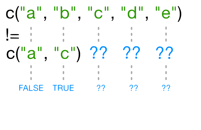
論理ベクトルを使ってサブセットを取ることもできます：

R

x[c(FALSE, FALSE, TRUE, FALSE, TRUE)]

OUTPUT

  c   e
7.1 7.5

比較演算子（例：>、<、==）は論理ベクトルを生成するため、それを使ってベクトルを簡潔にサブセットできます。以下のステートメントは、前の例と同じ結果を返します。

R

x[x > 7]

OUTPUT

  c   e
7.1 7.5

このステートメントを分解すると、まず x>7 が評価されて論理ベクトル c(FALSE, FALSE, TRUE, FALSE, TRUE) が生成され、それに基づいて x の要素が選択されます。

名前によるインデックス操作を模倣するには、== を使うことができます（比較には = ではなく == を使用する必要がある点に注意）：

R

x[names(x) == "a"]

OUTPUT

  a
5.4

ヒント: 複数の論理条件の結合

複数の論理条件を結合したい場合があります。たとえば、特定の範囲内の寿命を持つアジアまたはヨーロッパに位置するすべての国を見つけたいとします。このような場合、R では論理ベクトルを結合するための以下の演算子を使用できます：

&（論理AND）: 左右がともに TRUE の場合に TRUE を返します。
|（論理OR）: 左右のいずれか、または両方が TRUE の場合に TRUE を返します。

& や | の代わりに && や || が使われることもありますが、これらはベクトルの最初の要素だけを見て残りを無視します。データ解析では、通常1文字の演算子（& や |）を使用し、2文字の演算子はプログラミング（ステートメントの実行を決定する際など）で使用してください。

!（論理NOT）: TRUE を FALSE に、FALSE を TRUE に変換します。単一の条件（例：!TRUE は FALSE になる）や、ベクトル全体（例：!c(TRUE, FALSE) は c(FALSE, TRUE) になる）を否定できます。

また、単一のベクトル内の要素を比較するために、all（すべての要素が TRUE の場合に TRUE を返す）や any（1つ以上の要素が TRUE の場合に TRUE を返す）関数を使用できます。

チャレンジ 2

以下のコードを用いて：

R

x <- c(5.4, 6.2, 7.1, 4.8, 7.5)
names(x) <- c('a', 'b', 'c', 'd', 'e')
print(x)

OUTPUT

  a   b   c   d   e
5.4 6.2 7.1 4.8 7.5

x から 4 より大きく 7 未満の値を返すサブセットコマンドを書いてください。

チャレンジ 2 の解答

R

x_subset <- x[x<7 & x>4]
print(x_subset)

OUTPUT

  a   b   d
5.4 6.2 4.8

ヒント: 重複する名前

1つのベクトル内で複数の要素が同じ名前を持つことも可能です（データフレームでは、列名が重複することはありますが、行名は一意である必要があります）。以下の例を考えてみてください：

R

x <- 1:3
x

OUTPUT

[1] 1 2 3

R

names(x) <- c('a', 'a', 'a')
x

OUTPUT

a a a
1 2 3

R

x['a']  # 最初の値のみを返す

OUTPUT

a
1

R

x[names(x) == 'a']  # すべての値を返す

OUTPUT

a a a
1 2 3

ヒント: 演算子に関するヘルプを得る方法

演算子を引用符で囲むことで、ヘルプを検索できます：
help("%in%") または ?"%in%"。

名前付き要素をスキップする

名前付き要素をスキップまたは削除するのは少し難しいです。文字列を否定してスキップしようとすると、R は「文字列を否定する方法が分からない」というやや分かりにくいエラーを出します：

R

x <- c(a=5.4, b=6.2, c=7.1, d=4.8, e=7.5) # もう一度その場でベクトルに名前を付ける
x[-"a"]

ERROR

Error in -"a": invalid argument to unary operator

しかし、!=（等しくない）演算子を使用して論理ベクトルを構築すれば、望む動作を実現できます：

R

x[names(x) != "a"]

OUTPUT

  b   c   d   e
6.2 7.1 4.8 7.5

複数の名前付きインデックスをスキップするのはさらに難しいです。例えば、"a" と "c" を削除しようとして次のように試みます：

R

x[names(x)!=c("a","c")]

WARNING

Warning in names(x) != c("a", "c"): longer object length is not a multiple of
shorter object length

OUTPUT

  b   c   d   e
6.2 7.1 4.8 7.5

R は何かをしましたが、警告を出しており、それが示す通り 間違った結果 を返しました（"c" 要素がまだベクトルに含まれています）。

!= がこの場合に何を実際にしているのかは、非常に良い質問です。

リサイクル

このコードの比較部分を見てみましょう：

R

names(x) != c("a", "c")

WARNING

Warning in names(x) != c("a", "c"): longer object length is not a multiple of
shorter object length

OUTPUT

[1] FALSE  TRUE  TRUE  TRUE  TRUE

names(x)[3] != "c" は明らかに偽なのに、なぜ R はこのベクトルの3番目の要素に TRUE を返すのでしょうか？
!= を使用すると、R は左辺の各要素を右辺の対応する要素と比較しようとします。左辺と右辺の長さが異なる場合はどうなりますか？

一方のベクトルがもう一方より短い場合、短いベクトルは リサイクル されます：

この場合、R は c("a", "c") を必要な回数だけ繰り返して names(x) と一致させます（例：c("a","c","a","c","a")）。
再利用された "a" が names(x) の3番目の要素と一致しないため、!= の結果が TRUE になります。

リサイクルによりこのような間違いが発生するのを防ぐには %in% 演算子を使用します。この演算子は左辺の各要素について、右辺の中にその要素が存在するかどうかを確認します。今回は値を除外したいので、! 演算子も使用します：

R

x[! names(x) %in% c("a","c") ]

OUTPUT

  b   d   e
6.2 4.8 7.5

チャレンジ 3

ベクトルの要素を、特定のリスト内のいずれかと一致させる操作は、データ解析で非常に一般的なタスクです。例えば、gapminder データセットには country と continent の変数がありますが、これらの間の情報は含まれていません。東南アジアの情報を抽出したいとします。このとき、どのようにして東南アジアのすべての国について TRUE、それ以外を FALSE とする論理ベクトルを作成しますか？

以下のデータを使用します：

R

seAsia <- c("Myanmar","Thailand","Cambodia","Vietnam","Laos")
## エピソード2でダウンロードした gapminder データを読み込む
gapminder <- read.csv("data/gapminder_data.csv", header=TRUE)
## データフレームから `country` 列を抽出（詳細は後述）；
## factor を文字列に変換；
## 重複しない要素のみ取得
countries <- unique(as.character(gapminder$country))

以下の3つの方法を試し、それぞれがどのように（正しくない、または正しい方法で）動作するのか説明してください：

間違った方法（== のみを使用）
不格好な方法（論理演算子 == と | を使用）
エレガントな方法（%in% を使用）

チャレンジ 3 の解答

間違った方法
countries==seAsia
この方法では、警告（"In countries == seAsia : 長いオブジェクトの長さが短いオブジェクトの長さの倍数ではありません"）が表示され、誤った結果（すべて FALSE のベクトル）が返されます。これは、seAsia の再利用された値が正しい位置に一致しないためです。
不格好な方法
以下のコードでは正しい値を得ることができますが、非常に冗長で扱いにくいです：

R

 (countries=="Myanmar" | countries=="Thailand" |
 countries=="Cambodia" | countries == "Vietnam" | countries=="Laos")

または、countries==seAsia[1] | countries==seAsia[2] | ... のように記述します。
リストが長い場合、さらに複雑になります。

エレガントな方法
countries %in% seAsia
この方法は正確で、記述が簡単で可読性も高いです。

特殊値の扱い

R では、欠損値、無限値、未定義値を処理できない関数に出会うことがあります。
そのようなデータをフィルタリングするために、以下の特殊な関数を使用できます：

is.na：ベクトル、行列、またはデータフレーム内の NA（または NaN）を含む位置を返します。
同様に、is.nan と is.infinite は、それぞれ NaN と Inf に対応します。
is.finite：NA、NaN、Inf を含まない位置を返します。
na.omit：ベクトルからすべての欠損値を除外します。

因子のサブセット

ベクトルのサブセット方法を学んだところで、他のデータ構造のサブセットについて考えてみましょう。
因子のサブセットは、ベクトルのサブセットと同じ方法で行えます。

R

f <- factor(c("a", "a", "b", "c", "c", "d"))
f[f == "a"]

OUTPUT

[1] a a
Levels: a b c d

R

f[f %in% c("b", "c")]

OUTPUT

[1] b c c
Levels: a b c d

R

f[1:3]

OUTPUT

[1] a a b
Levels: a b c d

要素をスキップしても、そのカテゴリが因子レベルから削除されるわけではありません：

R

f[-3]

OUTPUT

[1] a a c c d
Levels: a b c d

行列のサブセット

行列は [ 関数を使用してサブセットします。この場合、2つの引数を取り、1つ目は行、2つ目は列に適用されます：

R

set.seed(1)
m <- matrix(rnorm(6*4), ncol=4, nrow=6)
m[3:4, c(3,1)]

OUTPUT

            [,1]       [,2]
[1,]  1.12493092 -0.8356286
[2,] -0.04493361  1.5952808

行または列全体を取得する場合は、1つ目または2つ目の引数を空白のままにします：

R

m[, c(3,4)]

OUTPUT

            [,1]        [,2]
[1,] -0.62124058  0.82122120
[2,] -2.21469989  0.59390132
[3,]  1.12493092  0.91897737
[4,] -0.04493361  0.78213630
[5,] -0.01619026  0.07456498
[6,]  0.94383621 -1.98935170

1つの行または列のみを取得すると、結果が自動的にベクトルに変換されます：

R

m[3,]

OUTPUT

[1] -0.8356286  0.5757814  1.1249309  0.9189774

結果を行列として保持するには、第3引数 を指定して drop = FALSE を設定します：

R

m[3, , drop=FALSE]

OUTPUT

           [,1]      [,2]     [,3]      [,4]
[1,] -0.8356286 0.5757814 1.124931 0.9189774

行または列の外側をアクセスしようとすると、R はエラーをスローします：

R

m[, c(3,6)]

ERROR

Error in m[, c(3, 6)]: subscript out of bounds

ヒント: 高次元配列

多次元配列の場合、[ の各引数が次元に対応します。例えば、3次元配列の場合、最初の3つの引数が行、列、および深さ次元に対応します。

行列はベクトルであるため、1つの引数だけを使用してサブセットを取ることもできます：

R

m[5]

OUTPUT

[1] 0.3295078

これは通常あまり有用ではなく、読み取りづらい場合があります。ただし、行列がデフォルトで 列優先フォーマット に配置されていることを理解するのに役立ちます。つまり、ベクトルの要素は列ごとに配置されます：

R

matrix(1:6, nrow=2, ncol=3)

OUTPUT

     [,1] [,2] [,3]
[1,]    1    3    5
[2,]    2    4    6

行ごとに行列を埋めたい場合は、byrow=TRUE を使用します：

R

matrix(1:6, nrow=2, ncol=3, byrow=TRUE)

OUTPUT

     [,1] [,2] [,3]
[1,]    1    2    3
[2,]    4    5    6

行列は、行および列のインデックスの代わりに、その行名および列名を使用してサブセットを取ることもできます。

チャレンジ 4

以下のコードを用いて：

R

m <- matrix(1:18, nrow=3, ncol=6)
print(m)

OUTPUT

     [,1] [,2] [,3] [,4] [,5] [,6]
[1,]    1    4    7   10   13   16
[2,]    2    5    8   11   14   17
[3,]    3    6    9   12   15   18

以下のコマンドのうち、11 と 14 を抽出するものはどれでしょうか？

A. m[2,4,2,5]
B. m[2:5]
C. m[4:5,2]
D. m[2,c(4,5)]

チャレンジ 4 の解答

リストのサブセット

ここでは新しいサブセット演算子を紹介します。リストをサブセットするためには、3つの関数を使用します。これらは、原子ベクトルや行列を学ぶ際にも登場しました：[, [[, $ です。

[ を使用すると、常にリストが返されます。リストから要素を「抽出」するのではなく「サブセット」したい場合に使用します。

R

xlist <- list(a = "Software Carpentry", b = 1:10, data = head(mtcars))
xlist[1]

OUTPUT

$a
[1] "Software Carpentry"

このコードは、1つの要素を含むリスト を返します。

リストの要素は、原子ベクトルと同じ方法でサブセットできます。ただし、比較演算は再帰的ではなく、リスト内のデータ構造に基づいて条件が評価されるため、リスト内の個々の要素には適用されません。

R

xlist[1:2]

OUTPUT

$a
[1] "Software Carpentry"

$b
 [1]  1  2  3  4  5  6  7  8  9 10

リストの個々の要素を抽出するには、二重角括弧関数 [[ を使用する必要があります。

R

xlist[[1]]

OUTPUT

[1] "Software Carpentry"

この結果はリストではなくベクトルであることに注意してください。

複数の要素を一度に抽出することはできません：

R

xlist[[1:2]]

ERROR

Error in xlist[[1:2]]: subscript out of bounds

また、要素をスキップすることもできません：

R

xlist[[-1]]

ERROR

Error in xlist[[-1]]: invalid negative subscript in get1index <real>

ただし、名前を使用して要素をサブセットおよび抽出することは可能です：

R

xlist[["a"]]

OUTPUT

[1] "Software Carpentry"

$ 演算子は、名前で要素を抽出するための簡潔な記法を提供します：

R

xlist$data

OUTPUT

                   mpg cyl disp  hp drat    wt  qsec vs am gear carb
Mazda RX4         21.0   6  160 110 3.90 2.620 16.46  0  1    4    4
Mazda RX4 Wag     21.0   6  160 110 3.90 2.875 17.02  0  1    4    4
Datsun 710        22.8   4  108  93 3.85 2.320 18.61  1  1    4    1
Hornet 4 Drive    21.4   6  258 110 3.08 3.215 19.44  1  0    3    1
Hornet Sportabout 18.7   8  360 175 3.15 3.440 17.02  0  0    3    2
Valiant           18.1   6  225 105 2.76 3.460 20.22  1  0    3    1

チャレンジ 5

以下のリストが与えられています：

R

xlist <- list(a = "Software Carpentry", b = 1:10, data = head(mtcars))

リストとベクトルのサブセット方法を用いて、xlist から数字の 2 を抽出してください。
ヒント：数字の 2 はリスト内の "b" に含まれています。

チャレンジ 5 の解答

R

xlist$b[2]

OUTPUT

[1] 2

R

xlist[[2]][2]

OUTPUT

[1] 2

R

xlist[["b"]][2]

OUTPUT

[1] 2

チャレンジ 6

以下の線形モデルが与えられています：

R

mod <- aov(pop ~ lifeExp, data=gapminder)

残差の自由度を抽出してください（ヒント：attributes() が役立ちます）。

チャレンジ 6 の解答

R

attributes(mod) ## `df.residual` は `mod` の名前の1つです

R

mod$df.residual

データフレーム

データフレームは内部的にはリストであることを覚えておきましょう。そのため、同様のルールが適用されます。ただし、データフレームは2次元のオブジェクトでもあります：

[ に1つの引数を与える場合、リストと同様に動作し、それぞれのリスト要素が列に対応します。結果として得られるオブジェクトはデータフレームになります：

R

head(gapminder[3])

OUTPUT

同様に、[[ を使用すると、単一の列 を抽出します：

R

head(gapminder[["lifeExp"]])

OUTPUT

[1] 28.801 30.332 31.997 34.020 36.088 38.438

$ 演算子は、列を名前で抽出するための便利なショートカットを提供します：

R

head(gapminder$year)

OUTPUT

[1] 1952 1957 1962 1967 1972 1977

2つの引数を与えると、[ は行列と同じように動作します：

R

gapminder[1:3,]

OUTPUT

      country year      pop continent lifeExp gdpPercap
1 Afghanistan 1952  8425333      Asia  28.801  779.4453
2 Afghanistan 1957  9240934      Asia  30.332  820.8530
3 Afghanistan 1962 10267083      Asia  31.997  853.1007

単一行をサブセットすると、結果はデータフレームになります（要素が混合型のためです）：

R

gapminder[3,]

OUTPUT

      country year      pop continent lifeExp gdpPercap
3 Afghanistan 1962 10267083      Asia  31.997  853.1007

ただし、単一列をサブセットすると結果はベクトルになります（第3引数 drop = FALSE を指定することで変更可能）。

チャレンジ 7

以下の一般的なデータフレームサブセットエラーを修正してください：

年 1957 の観測値を抽出する

R

gapminder[gapminder$year = 1957,]

1列目から4列目以外のすべての列を抽出する

R

gapminder[,-1:4]

寿命が80年以上の行を抽出する

R

gapminder[gapminder$lifeExp > 80]

1行目と4列目、5列目（continent と lifeExp）を抽出する

R

gapminder[1, 4, 5]

応用：年 2002 年と 2007 年の情報を含む行を抽出する

R

gapminder[gapminder$year == 2002 | 2007,]

チャレンジ 7 の解答

以下の一般的なデータフレームサブセットエラーを修正：

年 1957 の観測値を抽出する

R

# gapminder[gapminder$year = 1957,]
gapminder[gapminder$year == 1957,]

1列目から4列目以外のすべての列を抽出する

R

# gapminder[,-1:4]
gapminder[,-c(1:4)]

寿命が80年以上の行を抽出する

R

# gapminder[gapminder$lifeExp > 80]
gapminder[gapminder$lifeExp > 80,]

1行目と4列目、5列目（continent と lifeExp）を抽出する

R

# gapminder[1, 4, 5]
gapminder[1, c(4, 5)]

応用：年 2002 年と 2007 年の情報を含む行を抽出する

R

# gapminder[gapminder$year == 2002 | 2007,]
gapminder[gapminder$year == 2002 | gapminder$year == 2007,]
gapminder[gapminder$year %in% c(2002, 2007),]

Challenge 8

Why does gapminder[1:20] return an error? How does it differ from gapminder[1:20, ]?
Create a new data.frame called gapminder_small that only contains rows 1 through 9 and 19 through 23. You can do this in one or two steps.

Solution to challenge 8

gapminder is a data.frame so needs to be subsetted on two dimensions. gapminder[1:20, ] subsets the data to give the first 20 rows and all columns.

R

gapminder_small <- gapminder[c(1:9, 19:23),]

Key Points

Indexing in R starts at 1, not 0.
Access individual values by location using [].
Access slices of data using [low:high].
Access arbitrary sets of data using [c(...)].
Use logical operations and logical vectors to access subsets of data.

Content from Control Flow

Last updated on 2025-07-01 | Edit this page

Estimated time: 65 minutes

Overview

Questions

How can I make data-dependent choices in R?
How can I repeat operations in R?

Objectives

Write conditional statements with if...else statements and ifelse().
Write and understand for() loops.

Often when we’re coding we want to control the flow of our actions. This can be done by setting actions to occur only if a condition or a set of conditions are met. Alternatively, we can also set an action to occur a particular number of times.

There are several ways you can control flow in R. For conditional statements, the most commonly used approaches are the constructs:

R

# if
if (condition is true) {
  perform action
}

# if ... else
if (condition is true) {
  perform action
} else {  # that is, if the condition is false,
  perform alternative action
}

Say, for example, that we want R to print a message if a variable x has a particular value:

R

x <- 8

if (x >= 10) {
  print("x is greater than or equal to 10")
}

x

OUTPUT

[1] 8

The print statement does not appear in the console because x is not greater than 10. To print a different message for numbers less than 10, we can add an else statement.

R

x <- 8

if (x >= 10) {
  print("x is greater than or equal to 10")
} else {
  print("x is less than 10")
}

OUTPUT

[1] "x is less than 10"

You can also test multiple conditions by using else if.

R

x <- 8

if (x >= 10) {
  print("x is greater than or equal to 10")
} else if (x > 5) {
  print("x is greater than 5, but less than 10")
} else {
  print("x is less than 5")
}

OUTPUT

[1] "x is greater than 5, but less than 10"

Important: when R evaluates the condition inside if() statements, it is looking for a logical element, i.e., TRUE or FALSE. This can cause some headaches for beginners. For example:

R

x  <-  4 == 3
if (x) {
  "4 equals 3"
} else {
  "4 does not equal 3"
}

OUTPUT

[1] "4 does not equal 3"

As we can see, the not equal message was printed because the vector x is FALSE

R

x <- 4 == 3
x

OUTPUT

[1] FALSE

Challenge 1

Use an if() statement to print a suitable message reporting whether there are any records from 2002 in the gapminder dataset. Now do the same for 2012.

Solution to Challenge 1

We will first see a solution to Challenge 1 which does not use the any() function. We first obtain a logical vector describing which element of gapminder$year is equal to 2002:

R

gapminder[(gapminder$year == 2002),]

Then, we count the number of rows of the data.frame gapminder that correspond to the 2002:

R

rows2002_number <- nrow(gapminder[(gapminder$year == 2002),])

The presence of any record for the year 2002 is equivalent to the request that rows2002_number is one or more:

R

rows2002_number >= 1

Putting all together, we obtain:

R

if(nrow(gapminder[(gapminder$year == 2002),]) >= 1){
   print("Record(s) for the year 2002 found.")
}

All this can be done more quickly with any(). The logical condition can be expressed as:

R

if(any(gapminder$year == 2002)){
   print("Record(s) for the year 2002 found.")
}

Did anyone get a warning message like this?

ERROR

Error in if (gapminder$year == 2012) {: the condition has length > 1

The if() function only accepts singular (of length 1) inputs, and therefore returns an error when you use it with a vector. The if() function will still run, but will only evaluate the condition in the first element of the vector. Therefore, to use the if() function, you need to make sure your input is singular (of length 1).

Tip: Built in `ifelse()` function

R accepts both if() and else if() statements structured as outlined above, but also statements using R’s built-in ifelse() function. This function accepts both singular and vector inputs and is structured as follows:

R

# ifelse function
ifelse(condition is true, perform action, perform alternative action)

where the first argument is the condition or a set of conditions to be met, the second argument is the statement that is evaluated when the condition is TRUE, and the third statement is the statement that is evaluated when the condition is FALSE.

R

y <- -3
ifelse(y < 0, "y is a negative number", "y is either positive or zero")

OUTPUT

[1] "y is a negative number"

Tip: `any()` and `all()`

The any() function will return TRUE if at least one TRUE value is found within a vector, otherwise it will return FALSE. This can be used in a similar way to the %in% operator. The function all(), as the name suggests, will only return TRUE if all values in the vector are TRUE.

Repeating operations

If you want to iterate over a set of values, when the order of iteration is important, and perform the same operation on each, a for() loop will do the job. We saw for() loops in the shell lessons earlier. This is the most flexible of looping operations, but therefore also the hardest to use correctly. In general, the advice of many R users would be to learn about for() loops, but to avoid using for() loops unless the order of iteration is important: i.e. the calculation at each iteration depends on the results of previous iterations. If the order of iteration is not important, then you should learn about vectorized alternatives, such as the purrr package, as they pay off in computational efficiency.

The basic structure of a for() loop is:

R

for (iterator in set of values) {
  do a thing
}

For example:

R

for (i in 1:10) {
  print(i)
}

OUTPUT

[1] 1
[1] 2
[1] 3
[1] 4
[1] 5
[1] 6
[1] 7
[1] 8
[1] 9
[1] 10

The 1:10 bit creates a vector on the fly; you can iterate over any other vector as well.

We can use a for() loop nested within another for() loop to iterate over two things at once.

R

for (i in 1:5) {
  for (j in c('a', 'b', 'c', 'd', 'e')) {
    print(paste(i,j))
  }
}

OUTPUT

[1] "1 a"
[1] "1 b"
[1] "1 c"
[1] "1 d"
[1] "1 e"
[1] "2 a"
[1] "2 b"
[1] "2 c"
[1] "2 d"
[1] "2 e"
[1] "3 a"
[1] "3 b"
[1] "3 c"
[1] "3 d"
[1] "3 e"
[1] "4 a"
[1] "4 b"
[1] "4 c"
[1] "4 d"
[1] "4 e"
[1] "5 a"
[1] "5 b"
[1] "5 c"
[1] "5 d"
[1] "5 e"

We notice in the output that when the first index (i) is set to 1, the second index (j) iterates through its full set of indices. Once the indices of j have been iterated through, then i is incremented. This process continues until the last index has been used for each for() loop.

Rather than printing the results, we could write the loop output to a new object.

R

output_vector <- c()
for (i in 1:5) {
  for (j in c('a', 'b', 'c', 'd', 'e')) {
    temp_output <- paste(i, j)
    output_vector <- c(output_vector, temp_output)
  }
}
output_vector

OUTPUT

 [1] "1 a" "1 b" "1 c" "1 d" "1 e" "2 a" "2 b" "2 c" "2 d" "2 e" "3 a" "3 b"
[13] "3 c" "3 d" "3 e" "4 a" "4 b" "4 c" "4 d" "4 e" "5 a" "5 b" "5 c" "5 d"
[25] "5 e"

This approach can be useful, but ‘growing your results’ (building the result object incrementally) is computationally inefficient, so avoid it when you are iterating through a lot of values.

Tip: don’t grow your results

One of the biggest things that trips up novices and experienced R users alike, is building a results object (vector, list, matrix, data frame) as your for loop progresses. Computers are very bad at handling this, so your calculations can very quickly slow to a crawl. It’s much better to define an empty results object before hand of appropriate dimensions, rather than initializing an empty object without dimensions. So if you know the end result will be stored in a matrix like above, create an empty matrix with 5 row and 5 columns, then at each iteration store the results in the appropriate location.

A better way is to define your (empty) output object before filling in the values. For this example, it looks more involved, but is still more efficient.

R

output_matrix <- matrix(nrow = 5, ncol = 5)
j_vector <- c('a', 'b', 'c', 'd', 'e')
for (i in 1:5) {
  for (j in 1:5) {
    temp_j_value <- j_vector[j]
    temp_output <- paste(i, temp_j_value)
    output_matrix[i, j] <- temp_output
  }
}
output_vector2 <- as.vector(output_matrix)
output_vector2

OUTPUT

 [1] "1 a" "2 a" "3 a" "4 a" "5 a" "1 b" "2 b" "3 b" "4 b" "5 b" "1 c" "2 c"
[13] "3 c" "4 c" "5 c" "1 d" "2 d" "3 d" "4 d" "5 d" "1 e" "2 e" "3 e" "4 e"
[25] "5 e"

Tip: While loops

Sometimes you will find yourself needing to repeat an operation as long as a certain condition is met. You can do this with a while() loop.

R

while(this condition is true){
  do a thing
}

R will interpret a condition being met as “TRUE”.

As an example, here’s a while loop that generates random numbers from a uniform distribution (the runif() function) between 0 and 1 until it gets one that’s less than 0.1.

R

z <- 1
while(z > 0.1){
  z <- runif(1)
  cat(z, "\n")
}

while() loops will not always be appropriate. You have to be particularly careful that you don’t end up stuck in an infinite loop because your condition is always met and hence the while statement never terminates.

Challenge 2

Compare the objects output_vector and output_vector2. Are they the same? If not, why not? How would you change the last block of code to make output_vector2 the same as output_vector?

Solution to Challenge 2

We can check whether the two vectors are identical using the all() function:

R

all(output_vector == output_vector2)

However, all the elements of output_vector can be found in output_vector2:

R

all(output_vector %in% output_vector2)

and vice versa:

R

all(output_vector2 %in% output_vector)

therefore, the element in output_vector and output_vector2 are just sorted in a different order. This is because as.vector() outputs the elements of an input matrix going over its column. Taking a look at output_matrix, we can notice that we want its elements by rows. The solution is to transpose the output_matrix. We can do it either by calling the transpose function t() or by inputting the elements in the right order. The first solution requires to change the original

R

output_vector2 <- as.vector(output_matrix)

into

R

output_vector2 <- as.vector(t(output_matrix))

The second solution requires to change

R

output_matrix[i, j] <- temp_output

into

R

output_matrix[j, i] <- temp_output

Challenge 3

Write a script that loops through the gapminder data by continent and prints out whether the mean life expectancy is smaller or larger than 50 years.

Solution to Challenge 3

Step 1: We want to make sure we can extract all the unique values of the continent vector

R

gapminder <- read.csv("data/gapminder_data.csv")
unique(gapminder$continent)

Step 2: We also need to loop over each of these continents and calculate the average life expectancy for each subset of data. We can do that as follows:

Loop over each of the unique values of ‘continent’
For each value of continent, create a temporary variable storing that subset
Return the calculated life expectancy to the user by printing the output:

R

for (iContinent in unique(gapminder$continent)) {
  tmp <- gapminder[gapminder$continent == iContinent, ]
  cat(iContinent, mean(tmp$lifeExp, na.rm = TRUE), "\n")
  rm(tmp)
}

Step 3: The exercise only wants the output printed if the average life expectancy is less than 50 or greater than 50. So we need to add an if() condition before printing, which evaluates whether the calculated average life expectancy is above or below a threshold, and prints an output conditional on the result. We need to amend (3) from above:

3a. If the calculated life expectancy is less than some threshold (50 years), return the continent and a statement that life expectancy is less than threshold, otherwise return the continent and a statement that life expectancy is greater than threshold:

R

thresholdValue <- 50

for (iContinent in unique(gapminder$continent)) {
   tmp <- mean(gapminder[gapminder$continent == iContinent, "lifeExp"])

   if (tmp < thresholdValue){
       cat("Average Life Expectancy in", iContinent, "is less than", thresholdValue, "\n")
   } else {
       cat("Average Life Expectancy in", iContinent, "is greater than", thresholdValue, "\n")
   } # end if else condition
   rm(tmp)
} # end for loop

Challenge 4

Modify the script from Challenge 3 to loop over each country. This time print out whether the life expectancy is smaller than 50, between 50 and 70, or greater than 70.

Solution to Challenge 4

We modify our solution to Challenge 3 by now adding two thresholds, lowerThreshold and upperThreshold and extending our if-else statements:

R

 lowerThreshold <- 50
 upperThreshold <- 70

for (iCountry in unique(gapminder$country)) {
    tmp <- mean(gapminder[gapminder$country == iCountry, "lifeExp"])

    if(tmp < lowerThreshold) {
        cat("Average Life Expectancy in", iCountry, "is less than", lowerThreshold, "\n")
    } else if(tmp > lowerThreshold && tmp < upperThreshold) {
        cat("Average Life Expectancy in", iCountry, "is between", lowerThreshold, "and", upperThreshold, "\n")
    } else {
        cat("Average Life Expectancy in", iCountry, "is greater than", upperThreshold, "\n")
    }
    rm(tmp)
}

Challenge 5 - Advanced

Write a script that loops over each country in the gapminder dataset, tests whether the country starts with a ‘B’, and graphs life expectancy against time as a line graph if the mean life expectancy is under 50 years.

Solution for Challenge 5

We will use the grep() command that was introduced in the Unix Shell lesson to find countries that start with “B.” Lets understand how to do this first. Following from the Unix shell section we may be tempted to try the following

R

grep("^B", unique(gapminder$country))

But when we evaluate this command it returns the indices of the factor variable country that start with “B.” To get the values, we must add the value=TRUE option to the grep() command:

R

grep("^B", unique(gapminder$country), value = TRUE)

We will now store these countries in a variable called candidateCountries, and then loop over each entry in the variable. Inside the loop, we evaluate the average life expectancy for each country, and if the average life expectancy is less than 50 we use base-plot to plot the evolution of average life expectancy using with() and subset():

R

thresholdValue <- 50
candidateCountries <- grep("^B", unique(gapminder$country), value = TRUE)

for (iCountry in candidateCountries) {
    tmp <- mean(gapminder[gapminder$country == iCountry, "lifeExp"])

    if (tmp < thresholdValue) {
        cat("Average Life Expectancy in", iCountry, "is less than", thresholdValue, "plotting life expectancy graph... \n")

        with(subset(gapminder, country == iCountry),
                plot(year, lifeExp,
                     type = "o",
                     main = paste("Life Expectancy in", iCountry, "over time"),
                     ylab = "Life Expectancy",
                     xlab = "Year"
                     ) # end plot
             ) # end with
    } # end if
    rm(tmp)
} # end for loop

Key Points

Use if and else to make choices.
Use for to repeat operations.

Content from Creating Publication-Quality Graphics with ggplot2

Last updated on 2025-07-01 | Edit this page

Estimated time: 80 minutes

Overview

Questions

How can I create publication-quality graphics in R?

Objectives

To be able to use ggplot2 to generate publication-quality graphics.
To apply geometry, aesthetic, and statistics layers to a ggplot plot.
To manipulate the aesthetics of a plot using different colors, shapes, and lines.
To improve data visualization through transforming scales and paneling by group.
To save a plot created with ggplot to disk.

Plotting our data is one of the best ways to quickly explore it and the various relationships between variables.

There are three main plotting systems in R, the base plotting system, the lattice package, and the ggplot2 package.

Today we’ll be learning about the ggplot2 package, because it is the most effective for creating publication-quality graphics.

ggplot2 is built on the grammar of graphics, the idea that any plot can be built from the same set of components: a data set, mapping aesthetics, and graphical layers:

Data sets are the data that you, the user, provide.
Mapping aesthetics are what connect the data to the graphics. They tell ggplot2 how to use your data to affect how the graph looks, such as changing what is plotted on the X or Y axis, or the size or color of different data points.
Layers are the actual graphical output from ggplot2. Layers determine what kinds of plot are shown (scatterplot, histogram, etc.), the coordinate system used (rectangular, polar, others), and other important aspects of the plot. The idea of layers of graphics may be familiar to you if you have used image editing programs like Photoshop, Illustrator, or Inkscape.

Let’s start off building an example using the gapminder data from earlier. The most basic function is ggplot, which lets R know that we’re creating a new plot. Any of the arguments we give the ggplot function are the global options for the plot: they apply to all layers on the plot.

R

library("ggplot2")
ggplot(data = gapminder)

Blank plot, before adding any mapping aesthetics to ggplot().

Here we called ggplot and told it what data we want to show on our figure. This is not enough information for ggplot to actually draw anything. It only creates a blank slate for other elements to be added to.

Now we’re going to add in the mapping aesthetics using the aes function. aes tells ggplot how variables in the data map to aesthetic properties of the figure, such as which columns of the data should be used for the x and y locations.

R

ggplot(data = gapminder, mapping = aes(x = gdpPercap, y = lifeExp))

Plotting area with axes for a scatter plot of life expectancy vs GDP, with no data points visible.

Here we told ggplot we want to plot the “gdpPercap” column of the gapminder data frame on the x-axis, and the “lifeExp” column on the y-axis. Notice that we didn’t need to explicitly pass aes these columns (e.g. x = gapminder[, "gdpPercap"]), this is because ggplot is smart enough to know to look in the data for that column!

The final part of making our plot is to tell ggplot how we want to visually represent the data. We do this by adding a new layer to the plot using one of the geom functions.

R

ggplot(data = gapminder, mapping = aes(x = gdpPercap, y = lifeExp)) +
  geom_point()

Scatter plot of life expectancy vs GDP per capita, now showing the data points.

Here we used geom_point, which tells ggplot we want to visually represent the relationship between x and y as a scatterplot of points.

Challenge 1

Modify the example so that the figure shows how life expectancy has changed over time:

R

ggplot(data = gapminder, mapping = aes(x = gdpPercap, y = lifeExp)) + geom_point()

Hint: the gapminder dataset has a column called “year”, which should appear on the x-axis.

Solution to challenge 1

Here is one possible solution:

R

ggplot(data = gapminder, mapping = aes(x = year, y = lifeExp)) + geom_point()

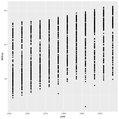
Binned scatterplot of life expectancy versus year showing how life expectancy has increased over time

Challenge 2

In the previous examples and challenge we’ve used the aes function to tell the scatterplot geom about the x and y locations of each point. Another aesthetic property we can modify is the point color. Modify the code from the previous challenge to color the points by the “continent” column. What trends do you see in the data? Are they what you expected?

Solution to challenge 2

The solution presented below adds color=continent to the call of the aes function. The general trend seems to indicate an increased life expectancy over the years. On continents with stronger economies we find a longer life expectancy.

R

ggplot(data = gapminder, mapping = aes(x = year, y = lifeExp, color=continent)) +
  geom_point()

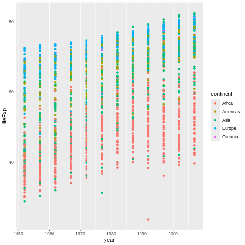
Binned scatterplot of life expectancy vs year with color-coded continents showing value of 'aes' function — Binned scatterplot of life expectancy vs year with color-coded continents showing value of ‘aes’ function

Layers

Using a scatterplot probably isn’t the best for visualizing change over time. Instead, let’s tell ggplot to visualize the data as a line plot:

R

ggplot(data = gapminder, mapping = aes(x=year, y=lifeExp, color=continent)) +
  geom_line()

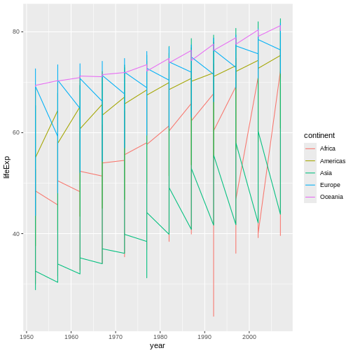
Instead of adding a geom_point layer, we’ve added a geom_line layer.

However, the result doesn’t look quite as we might have expected: it seems to be jumping around a lot in each continent. Let’s try to separate the data by country, plotting one line for each country:

R

ggplot(data = gapminder, mapping = aes(x=year, y=lifeExp, group=country, color=continent)) +
  geom_line()

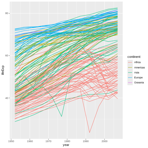
We’ve added the group aesthetic, which tells ggplot to draw a line for each country.

But what if we want to visualize both lines and points on the plot? We can add another layer to the plot:

R

ggplot(data = gapminder, mapping = aes(x=year, y=lifeExp, group=country, color=continent)) +
  geom_line() + geom_point()

It’s important to note that each layer is drawn on top of the previous layer. In this example, the points have been drawn on top of the lines. Here’s a demonstration:

R

ggplot(data = gapminder, mapping = aes(x=year, y=lifeExp, group=country)) +
  geom_line(mapping = aes(color=continent)) + geom_point()

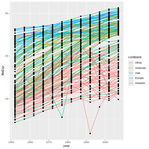
In this example, the aesthetic mapping of color has been moved from the global plot options in ggplot to the geom_line layer so it no longer applies to the points. Now we can clearly see that the points are drawn on top of the lines.

Tip: Setting an aesthetic to a value instead of a mapping

So far, we’ve seen how to use an aesthetic (such as color) as a mapping to a variable in the data. For example, when we use geom_line(mapping = aes(color=continent)), ggplot will give a different color to each continent. But what if we want to change the color of all lines to blue? You may think that geom_line(mapping = aes(color="blue")) should work, but it doesn’t. Since we don’t want to create a mapping to a specific variable, we can move the color specification outside of the aes() function, like this: geom_line(color="blue").

Challenge 3

Switch the order of the point and line layers from the previous example. What happened?

Solution to challenge 3

The lines now get drawn over the points!

R

ggplot(data = gapminder, mapping = aes(x=year, y=lifeExp, group=country)) +
 geom_point() + geom_line(mapping = aes(color=continent))

Scatter plot of life expectancy vs GDP per capita with a trend line summarising the relationship between variables. The plot illustrates the possibilities for styling visualisations in ggplot2 with data points enlarged, coloured orange, and displayed without transparency.

Transformations and statistics

ggplot2 also makes it easy to overlay statistical models over the data. To demonstrate we’ll go back to our first example:

R

ggplot(data = gapminder, mapping = aes(x = gdpPercap, y = lifeExp)) +
  geom_point()

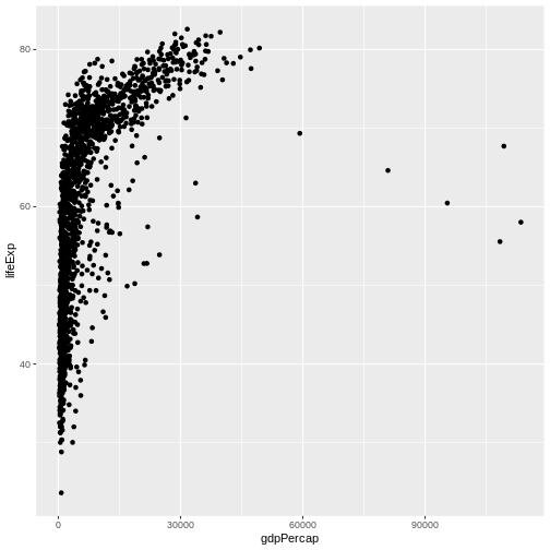
Currently it’s hard to see the relationship between the points due to some strong outliers in GDP per capita. We can change the scale of units on the x axis using the scale functions. These control the mapping between the data values and visual values of an aesthetic. We can also modify the transparency of the points, using the alpha function, which is especially helpful when you have a large amount of data which is very clustered.

R

ggplot(data = gapminder, mapping = aes(x = gdpPercap, y = lifeExp)) +
  geom_point(alpha = 0.5) + scale_x_log10()

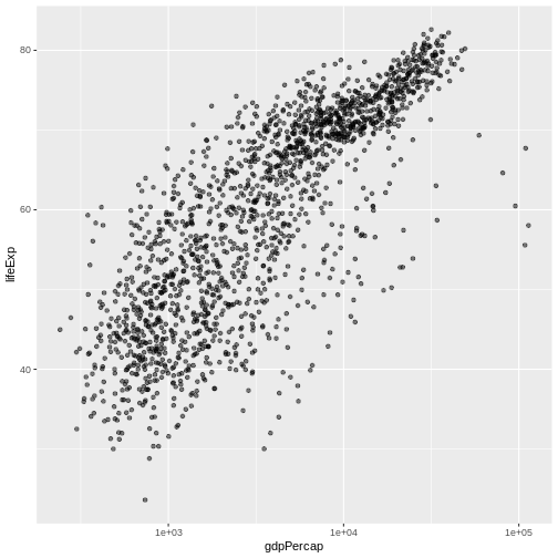
Scatterplot of GDP vs life expectancy showing logarithmic x-axis data spread

The scale_x_log10 function applied a transformation to the coordinate system of the plot, so that each multiple of 10 is evenly spaced from left to right. For example, a GDP per capita of 1,000 is the same horizontal distance away from a value of 10,000 as the 10,000 value is from 100,000. This helps to visualize the spread of the data along the x-axis.

Tip Reminder: Setting an aesthetic to a value instead of a mapping

Notice that we used geom_point(alpha = 0.5). As the previous tip mentioned, using a setting outside of the aes() function will cause this value to be used for all points, which is what we want in this case. But just like any other aesthetic setting, alpha can also be mapped to a variable in the data. For example, we can give a different transparency to each continent with geom_point(mapping = aes(alpha = continent)).

We can fit a simple relationship to the data by adding another layer, geom_smooth:

R

ggplot(data = gapminder, mapping = aes(x = gdpPercap, y = lifeExp)) +
  geom_point(alpha = 0.5) + scale_x_log10() + geom_smooth(method="lm")

OUTPUT

`geom_smooth()` using formula = 'y ~ x'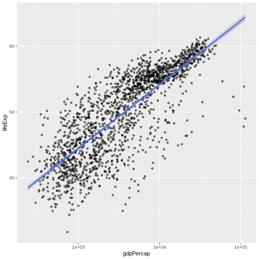

Scatter plot of life expectancy vs GDP per capita with a blue trend line summarising the relationship between variables, and gray shaded area indicating 95% confidence intervals for that trend line.

We can make the line thicker by setting the linewidth aesthetic in the geom_smooth layer:

R

ggplot(data = gapminder, mapping = aes(x = gdpPercap, y = lifeExp)) +
  geom_point(alpha = 0.5) + scale_x_log10() + geom_smooth(method="lm", linewidth=1.5)

OUTPUT

`geom_smooth()` using formula = 'y ~ x'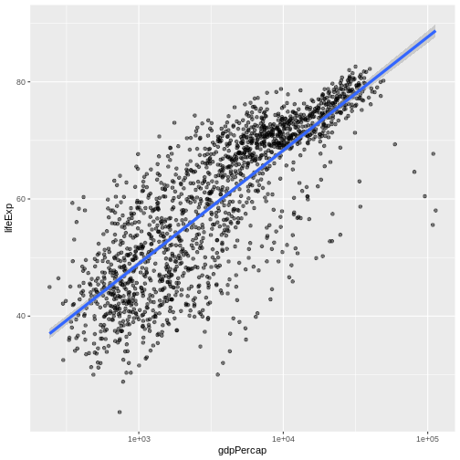

Scatter plot of life expectancy vs GDP per capita with a trend line summarising the relationship between variables. The blue trend line is slightly thicker than in the previous figure.

There are two ways an aesthetic can be specified. Here we set the linewidth aesthetic by passing it as an argument to geom_smooth and it is applied the same to the whole geom. Previously in the lesson we’ve used the aes function to define a mapping between data variables and their visual representation.

Challenge 4a

Modify the color and size of the points on the point layer in the previous example.

Hint: do not use the aes function.

Hint: the equivalent of linewidth for points is size.

Solution to challenge 4a

Here a possible solution: Notice that the color argument is supplied outside of the aes() function. This means that it applies to all data points on the graph and is not related to a specific variable.

R

ggplot(data = gapminder, mapping = aes(x = gdpPercap, y = lifeExp)) +
 geom_point(size=3, color="orange") + scale_x_log10() +
 geom_smooth(method="lm", linewidth=1.5)

OUTPUT

`geom_smooth()` using formula = 'y ~ x'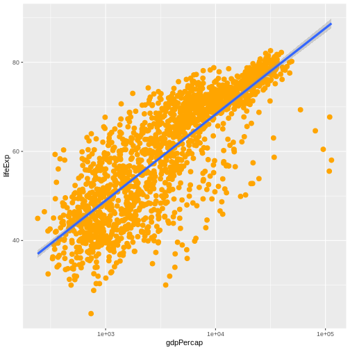

Challenge 4b

Modify your solution to Challenge 4a so that the points are now a different shape and are colored by continent with new trendlines. Hint: The color argument can be used inside the aesthetic.

Solution to challenge 4b

Here is a possible solution: Notice that supplying the color argument inside the aes() functions enables you to connect it to a certain variable. The shape argument, as you can see, modifies all data points the same way (it is outside the aes() call) while the color argument which is placed inside the aes() call modifies a point’s color based on its continent value.

R

ggplot(data = gapminder, mapping = aes(x = gdpPercap, y = lifeExp, color = continent)) +
 geom_point(size=3, shape=17) + scale_x_log10() +
 geom_smooth(method="lm", linewidth=1.5)

OUTPUT

`geom_smooth()` using formula = 'y ~ x'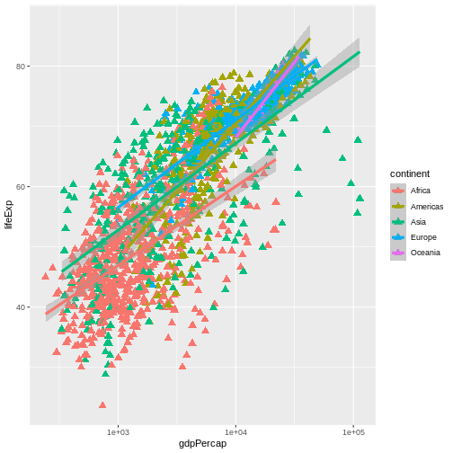

Multi-panel figures

Earlier we visualized the change in life expectancy over time across all countries in one plot. Alternatively, we can split this out over multiple panels by adding a layer of facet panels.

Tip

We start by making a subset of data including only countries located in the Americas. This includes 25 countries, which will begin to clutter the figure. Note that we apply a “theme” definition to rotate the x-axis labels to maintain readability. Nearly everything in ggplot2 is customizable.

R

americas <- gapminder[gapminder$continent == "Americas",]
ggplot(data = americas, mapping = aes(x = year, y = lifeExp)) +
  geom_line() +
  facet_wrap( ~ country) +
  theme(axis.text.x = element_text(angle = 45))

The facet_wrap layer took a “formula” as its argument, denoted by the tilde (~). This tells R to draw a panel for each unique value in the country column of the gapminder dataset.

Modifying text

To clean this figure up for a publication we need to change some of the text elements. The x-axis is too cluttered, and the y axis should read “Life expectancy”, rather than the column name in the data frame.

We can do this by adding a couple of different layers. The theme layer controls the axis text, and overall text size. Labels for the axes, plot title and any legend can be set using the labs function. Legend titles are set using the same names we used in the aes specification. Thus below the color legend title is set using color = "Continent", while the title of a fill legend would be set using fill = "MyTitle".

R

ggplot(data = americas, mapping = aes(x = year, y = lifeExp, color=continent)) +
  geom_line() + facet_wrap( ~ country) +
  labs(
    x = "Year",              # x axis title
    y = "Life expectancy",   # y axis title
    title = "Figure 1",      # main title of figure
    color = "Continent"      # title of legend
  ) +
  theme(axis.text.x = element_text(angle = 90, hjust = 1))

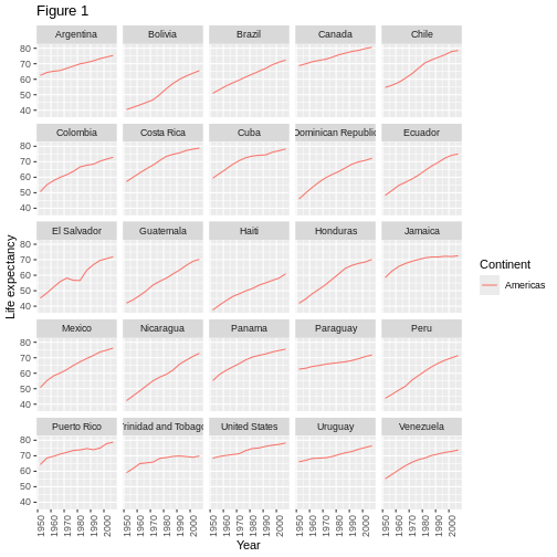
Exporting the plot

The ggsave() function allows you to export a plot created with ggplot. You can specify the dimension and resolution of your plot by adjusting the appropriate arguments (width, height and dpi) to create high quality graphics for publication. In order to save the plot from above, we first assign it to a variable lifeExp_plot, then tell ggsave to save that plot in png format to a directory called results. (Make sure you have a results/ folder in your working directory.)

R

lifeExp_plot <- ggplot(data = americas, mapping = aes(x = year, y = lifeExp, color=continent)) +
  geom_line() + facet_wrap( ~ country) +
  labs(
    x = "Year",              # x axis title
    y = "Life expectancy",   # y axis title
    title = "Figure 1",      # main title of figure
    color = "Continent"      # title of legend
  ) +
  theme(axis.text.x = element_text(angle = 90, hjust = 1))

ggsave(filename = "results/lifeExp.png", plot = lifeExp_plot, width = 12, height = 10, dpi = 300, units = "cm")

There are two nice things about ggsave. First, it defaults to the last plot, so if you omit the plot argument it will automatically save the last plot you created with ggplot. Secondly, it tries to determine the format you want to save your plot in from the file extension you provide for the filename (for example .png or .pdf). If you need to, you can specify the format explicitly in the device argument.

This is a taste of what you can do with ggplot2. RStudio provides a really useful cheat sheet of the different layers available, and more extensive documentation is available on the ggplot2 website. All RStudio cheat sheets are available from the RStudio website. Finally, if you have no idea how to change something, a quick Google search will usually send you to a relevant question and answer on Stack Overflow with reusable code to modify!

Challenge 5

Generate boxplots to compare life expectancy between the different continents during the available years.

Advanced:

Rename y axis as Life Expectancy.
Remove x axis labels.

Solution to Challenge 5

Here a possible solution: xlab() and ylab() set labels for the x and y axes, respectively The axis title, text and ticks are attributes of the theme and must be modified within a theme() call.

R

ggplot(data = gapminder, mapping = aes(x = continent, y = lifeExp, fill = continent)) +
 geom_boxplot() + facet_wrap(~year) +
 ylab("Life Expectancy") +
 theme(axis.title.x=element_blank(),
       axis.text.x = element_blank(),
       axis.ticks.x = element_blank())

Key Points

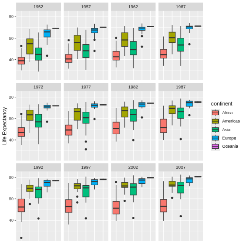
Use ggplot2 to create plots.
Think about graphics in layers: aesthetics, geometry, statistics, scale transformation, and grouping.

Content from Vectorization

Last updated on 2025-07-01 | Edit this page

Estimated time: 25 minutes

Overview

Questions

How can I operate on all the elements of a vector at once?

Objectives

To understand vectorized operations in R.

Most of R’s functions are vectorized, meaning that the function will operate on all elements of a vector without needing to loop through and act on each element one at a time. This makes writing code more concise, easy to read, and less error prone.

R

x <- 1:4
x * 2

OUTPUT

[1] 2 4 6 8

The multiplication happened to each element of the vector.

We can also add two vectors together:

R

y <- 6:9
x + y

OUTPUT

[1]  7  9 11 13

Each element of x was added to its corresponding element of y:

R

x:  1  2  3  4
    +  +  +  +
y:  6  7  8  9
---------------
    7  9 11 13

Here is how we would add two vectors together using a for loop:

R

output_vector <- c()
for (i in 1:4) {
  output_vector[i] <- x[i] + y[i]
}
output_vector

OUTPUT

[1]  7  9 11 13

Compare this to the output using vectorised operations.

R

sum_xy <- x + y
sum_xy

OUTPUT

[1]  7  9 11 13

Challenge 1

Let’s try this on the pop column of the gapminder dataset.

Make a new column in the gapminder data frame that contains population in units of millions of people. Check the head or tail of the data frame to make sure it worked.

Solution to challenge 1

Let’s try this on the pop column of the gapminder dataset.

Make a new column in the gapminder data frame that contains population in units of millions of people. Check the head or tail of the data frame to make sure it worked.

R

gapminder$pop_millions <- gapminder$pop / 1e6
head(gapminder)

OUTPUT

      country year      pop continent lifeExp gdpPercap pop_millions
1 Afghanistan 1952  8425333      Asia  28.801  779.4453     8.425333
2 Afghanistan 1957  9240934      Asia  30.332  820.8530     9.240934
3 Afghanistan 1962 10267083      Asia  31.997  853.1007    10.267083
4 Afghanistan 1967 11537966      Asia  34.020  836.1971    11.537966
5 Afghanistan 1972 13079460      Asia  36.088  739.9811    13.079460
6 Afghanistan 1977 14880372      Asia  38.438  786.1134    14.880372

Challenge 2

On a single graph, plot population, in millions, against year, for all countries. Do not worry about identifying which country is which.

Repeat the exercise, graphing only for China, India, and Indonesia. Again, do not worry about which is which.

Solution to challenge 2

Refresh your plotting skills by plotting population in millions against year.

R

ggplot(gapminder, aes(x = year, y = pop_millions)) +
 geom_point()

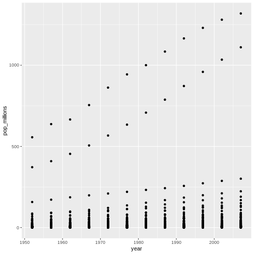
Scatter plot showing populations in the millions against the year for China, India, and Indonesia, countries are not labeled.

R

countryset <- c("China","India","Indonesia")
ggplot(gapminder[gapminder$country %in% countryset,],
       aes(x = year, y = pop_millions)) +
  geom_point()

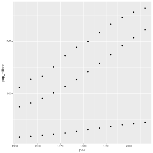
Comparison operators, logical operators, and many functions are also vectorized:

Comparison operators

R

x > 2

OUTPUT

[1] FALSE FALSE  TRUE  TRUE

Logical operators

R

a <- x > 3  # or, for clarity, a <- (x > 3)
a

OUTPUT

[1] FALSE FALSE FALSE  TRUE

Tip: some useful functions for logical vectors

any() will return TRUE if any element of a vector is TRUE.
all() will return TRUE if all elements of a vector are TRUE.

Most functions also operate element-wise on vectors:

Functions

R

x <- 1:4
log(x)

OUTPUT

[1] 0.0000000 0.6931472 1.0986123 1.3862944

Vectorized operations work element-wise on matrices:

R

m <- matrix(1:12, nrow=3, ncol=4)
m * -1

OUTPUT

     [,1] [,2] [,3] [,4]
[1,]   -1   -4   -7  -10
[2,]   -2   -5   -8  -11
[3,]   -3   -6   -9  -12

Tip: element-wise vs. matrix multiplication

Very important: the operator * gives you element-wise multiplication! To do matrix multiplication, we need to use the %*% operator:

R

m %*% matrix(1, nrow=4, ncol=1)

OUTPUT

     [,1]
[1,]   22
[2,]   26
[3,]   30

R

matrix(1:4, nrow=1) %*% matrix(1:4, ncol=1)

OUTPUT

     [,1]
[1,]   30

For more on matrix algebra, see the Quick-R reference guide

Challenge 3

Given the following matrix:

R

m <- matrix(1:12, nrow=3, ncol=4)
m

OUTPUT

     [,1] [,2] [,3] [,4]
[1,]    1    4    7   10
[2,]    2    5    8   11
[3,]    3    6    9   12

Write down what you think will happen when you run:

m ^ -1
m * c(1, 0, -1)
m > c(0, 20)
m * c(1, 0, -1, 2)

Did you get the output you expected? If not, ask a helper!

Solution to challenge 3

Given the following matrix:

R

m <- matrix(1:12, nrow=3, ncol=4)
m

OUTPUT

     [,1] [,2] [,3] [,4]
[1,]    1    4    7   10
[2,]    2    5    8   11
[3,]    3    6    9   12

Write down what you think will happen when you run:

m ^ -1

OUTPUT

          [,1]      [,2]      [,3]       [,4]
[1,] 1.0000000 0.2500000 0.1428571 0.10000000
[2,] 0.5000000 0.2000000 0.1250000 0.09090909
[3,] 0.3333333 0.1666667 0.1111111 0.08333333

m * c(1, 0, -1)

OUTPUT

     [,1] [,2] [,3] [,4]
[1,]    1    4    7   10
[2,]    0    0    0    0
[3,]   -3   -6   -9  -12

m > c(0, 20)

OUTPUT

      [,1]  [,2]  [,3]  [,4]
[1,]  TRUE FALSE  TRUE FALSE
[2,] FALSE  TRUE FALSE  TRUE
[3,]  TRUE FALSE  TRUE FALSE

Challenge 4

We’re interested in looking at the sum of the following sequence of fractions:

R

 x = 1/(1^2) + 1/(2^2) + 1/(3^2) + ... + 1/(n^2)

This would be tedious to type out, and impossible for high values of n. Use vectorisation to compute x when n=100. What is the sum when n=10,000?

Challenge 4

We’re interested in looking at the sum of the following sequence of fractions:

R

 x = 1/(1^2) + 1/(2^2) + 1/(3^2) + ... + 1/(n^2)

This would be tedious to type out, and impossible for high values of n. Can you use vectorisation to compute x, when n=100? How about when n=10,000?

R

sum(1/(1:100)^2)

OUTPUT

[1] 1.634984

R

sum(1/(1:1e04)^2)

OUTPUT

[1] 1.644834

R

n <- 10000
sum(1/(1:n)^2)

OUTPUT

[1] 1.644834

We can also obtain the same results using a function:

R

inverse_sum_of_squares <- function(n) {
  sum(1/(1:n)^2)
}
inverse_sum_of_squares(100)

OUTPUT

[1] 1.634984

R

inverse_sum_of_squares(10000)

OUTPUT

[1] 1.644834

R

n <- 10000
inverse_sum_of_squares(n)

OUTPUT

[1] 1.644834

Tip: Operations on vectors of unequal length

Operations can also be performed on vectors of unequal length, through a process known as recycling. This process automatically repeats the smaller vector until it matches the length of the larger vector. R will provide a warning if the larger vector is not a multiple of the smaller vector.

R

x <- c(1, 2, 3)
y <- c(1, 2, 3, 4, 5, 6, 7)
x + y

WARNING

Warning in x + y: longer object length is not a multiple of shorter object
length

OUTPUT

[1] 2 4 6 5 7 9 8

Vector x was recycled to match the length of vector y

R

x:  1  2  3  1  2  3  1
    +  +  +  +  +  +  +
y:  1  2  3  4  5  6  7
-----------------------
    2  4  6  5  7  9  8

Key Points

Use vectorized operations instead of loops.

Content from Functions Explained

Last updated on 2025-07-01 | Edit this page

Estimated time: 60 minutes

Overview

Questions

How can I write a new function in R?

Objectives

Define a function that takes arguments.
Return a value from a function.
Check argument conditions with stopifnot() in functions.
Test a function.
Set default values for function arguments.
Explain why we should divide programs into small, single-purpose functions.

If we only had one data set to analyze, it would probably be faster to load the file into a spreadsheet and use that to plot simple statistics. However, the gapminder data is updated periodically, and we may want to pull in that new information later and re-run our analysis again. We may also obtain similar data from a different source in the future.

In this lesson, we’ll learn how to write a function so that we can repeat several operations with a single command.

What is a function?

Functions gather a sequence of operations into a whole, preserving it for ongoing use. Functions provide:

a name we can remember and invoke it by
relief from the need to remember the individual operations
a defined set of inputs and expected outputs
rich connections to the larger programming environment

As the basic building block of most programming languages, user-defined functions constitute “programming” as much as any single abstraction can. If you have written a function, you are a computer programmer.

Defining a function

Let’s open a new R script file in the functions/ directory and call it functions-lesson.R.

The general structure of a function is:

R

my_function <- function(parameters) {
  # perform action
  # return value
}

Let’s define a function fahr_to_kelvin() that converts temperatures from Fahrenheit to Kelvin:

R

fahr_to_kelvin <- function(temp) {
  kelvin <- ((temp - 32) * (5 / 9)) + 273.15
  return(kelvin)
}

We define fahr_to_kelvin() by assigning it to the output of function. The list of argument names are contained within parentheses. Next, the body of the function–the statements that are executed when it runs–is contained within curly braces ({}). The statements in the body are indented by two spaces. This makes the code easier to read but does not affect how the code operates.

It is useful to think of creating functions like writing a cookbook. First you define the “ingredients” that your function needs. In this case, we only need one ingredient to use our function: “temp”. After we list our ingredients, we then say what we will do with them, in this case, we are taking our ingredient and applying a set of mathematical operators to it.

When we call the function, the values we pass to it as arguments are assigned to those variables so that we can use them inside the function. Inside the function, we use a return statement to send a result back to whoever asked for it.

Tip

One feature unique to R is that the return statement is not required. R automatically returns whichever variable is on the last line of the body of the function. But for clarity, we will explicitly define the return statement.

Let’s try running our function. Calling our own function is no different from calling any other function:

R

# freezing point of water
fahr_to_kelvin(32)

OUTPUT

[1] 273.15

R

# boiling point of water
fahr_to_kelvin(212)

OUTPUT

[1] 373.15

Challenge 1

Write a function called kelvin_to_celsius() that takes a temperature in Kelvin and returns that temperature in Celsius.

Hint: To convert from Kelvin to Celsius you subtract 273.15

Solution to challenge 1

Write a function called kelvin_to_celsius that takes a temperature in Kelvin and returns that temperature in Celsius

R

kelvin_to_celsius <- function(temp) {
 celsius <- temp - 273.15
 return(celsius)
}

Combining functions

The real power of functions comes from mixing, matching and combining them into ever-larger chunks to get the effect we want.

Let’s define two functions that will convert temperature from Fahrenheit to Kelvin, and Kelvin to Celsius:

R

fahr_to_kelvin <- function(temp) {
  kelvin <- ((temp - 32) * (5 / 9)) + 273.15
  return(kelvin)
}

kelvin_to_celsius <- function(temp) {
  celsius <- temp - 273.15
  return(celsius)
}

Challenge 2

Define the function to convert directly from Fahrenheit to Celsius, by reusing the two functions above (or using your own functions if you prefer).

Solution to challenge 2

Define the function to convert directly from Fahrenheit to Celsius, by reusing these two functions above

R

fahr_to_celsius <- function(temp) {
  temp_k <- fahr_to_kelvin(temp)
  result <- kelvin_to_celsius(temp_k)
  return(result)
}

Interlude: Defensive Programming

Now that we’ve begun to appreciate how writing functions provides an efficient way to make R code re-usable and modular, we should note that it is important to ensure that functions only work in their intended use-cases. Checking function parameters is related to the concept of defensive programming. Defensive programming encourages us to frequently check conditions and throw an error if something is wrong. These checks are referred to as assertion statements because we want to assert some condition is TRUE before proceeding. They make it easier to debug because they give us a better idea of where the errors originate.

Checking conditions with `stopifnot()`

Let’s start by re-examining fahr_to_kelvin(), our function for converting temperatures from Fahrenheit to Kelvin. It was defined like so:

R

fahr_to_kelvin <- function(temp) {
  kelvin <- ((temp - 32) * (5 / 9)) + 273.15
  return(kelvin)
}

For this function to work as intended, the argument temp must be a numeric value; otherwise, the mathematical procedure for converting between the two temperature scales will not work. To create an error, we can use the function stop(). For example, since the argument temp must be a numeric vector, we could check for this condition with an if statement and throw an error if the condition was violated. We could augment our function above like so:

R

fahr_to_kelvin <- function(temp) {
  if (!is.numeric(temp)) {
    stop("temp must be a numeric vector.")
  }
  kelvin <- ((temp - 32) * (5 / 9)) + 273.15
  return(kelvin)
}

If we had multiple conditions or arguments to check, it would take many lines of code to check all of them. Luckily R provides the convenience function stopifnot(). We can list as many requirements that should evaluate to TRUE; stopifnot() throws an error if it finds one that is FALSE. Listing these conditions also serves a secondary purpose as extra documentation for the function.

Let’s try out defensive programming with stopifnot() by adding assertions to check the input to our function fahr_to_kelvin().

We want to assert the following: temp is a numeric vector. We may do that like so:

R

fahr_to_kelvin <- function(temp) {
  stopifnot(is.numeric(temp))
  kelvin <- ((temp - 32) * (5 / 9)) + 273.15
  return(kelvin)
}

It still works when given proper input.

R

# freezing point of water
fahr_to_kelvin(temp = 32)

OUTPUT

[1] 273.15

But fails instantly if given improper input.

R

# Metric is a factor instead of numeric
fahr_to_kelvin(temp = as.factor(32))

ERROR

Error in fahr_to_kelvin(temp = as.factor(32)): is.numeric(temp) is not TRUE

Challenge 3

Use defensive programming to ensure that our fahr_to_celsius() function throws an error immediately if the argument temp is specified inappropriately.

Solution to challenge 3

Extend our previous definition of the function by adding in an explicit call to stopifnot(). Since fahr_to_celsius() is a composition of two other functions, checking inside here makes adding checks to the two component functions redundant.

R

fahr_to_celsius <- function(temp) {
  stopifnot(is.numeric(temp))
  temp_k <- fahr_to_kelvin(temp)
  result <- kelvin_to_celsius(temp_k)
  return(result)
}

More on combining functions

Now, we’re going to define a function that calculates the Gross Domestic Product of a nation from the data available in our dataset:

R

# Takes a dataset and multiplies the population column
# with the GDP per capita column.
calcGDP <- function(dat) {
  gdp <- dat$pop * dat$gdpPercap
  return(gdp)
}

We define calcGDP() by assigning it to the output of function. The list of argument names are contained within parentheses. Next, the body of the function -- the statements executed when you call the function – is contained within curly braces ({}).

We’ve indented the statements in the body by two spaces. This makes the code easier to read but does not affect how it operates.

When we call the function, the values we pass to it are assigned to the arguments, which become variables inside the body of the function.

Inside the function, we use the return() function to send back the result. This return() function is optional: R will automatically return the results of whatever command is executed on the last line of the function.

R

calcGDP(head(gapminder))

OUTPUT

[1]  6567086330  7585448670  8758855797  9648014150  9678553274 11697659231

That’s not very informative. Let’s add some more arguments so we can extract that per year and country.

R

# Takes a dataset and multiplies the population column
# with the GDP per capita column.
calcGDP <- function(dat, year=NULL, country=NULL) {
  if(!is.null(year)) {
    dat <- dat[dat$year %in% year, ]
  }
  if (!is.null(country)) {
    dat <- dat[dat$country %in% country,]
  }
  gdp <- dat$pop * dat$gdpPercap

  new <- cbind(dat, gdp=gdp)
  return(new)
}

If you’ve been writing these functions down into a separate R script (a good idea!), you can load in the functions into our R session by using the source() function:

R

source("functions/functions-lesson.R")

Ok, so there’s a lot going on in this function now. In plain English, the function now subsets the provided data by year if the year argument isn’t empty, then subsets the result by country if the country argument isn’t empty. Then it calculates the GDP for whatever subset emerges from the previous two steps. The function then adds the GDP as a new column to the subsetted data and returns this as the final result. You can see that the output is much more informative than a vector of numbers.

Let’s take a look at what happens when we specify the year:

R

head(calcGDP(gapminder, year=2007))

OUTPUT

       country year      pop continent lifeExp  gdpPercap          gdp
12 Afghanistan 2007 31889923      Asia  43.828   974.5803  31079291949
24     Albania 2007  3600523    Europe  76.423  5937.0295  21376411360
36     Algeria 2007 33333216    Africa  72.301  6223.3675 207444851958
48      Angola 2007 12420476    Africa  42.731  4797.2313  59583895818
60   Argentina 2007 40301927  Americas  75.320 12779.3796 515033625357
72   Australia 2007 20434176   Oceania  81.235 34435.3674 703658358894

Or for a specific country:

R

calcGDP(gapminder, country="Australia")

OUTPUT

     country year      pop continent lifeExp gdpPercap          gdp
61 Australia 1952  8691212   Oceania  69.120  10039.60  87256254102
62 Australia 1957  9712569   Oceania  70.330  10949.65 106349227169
63 Australia 1962 10794968   Oceania  70.930  12217.23 131884573002
64 Australia 1967 11872264   Oceania  71.100  14526.12 172457986742
65 Australia 1972 13177000   Oceania  71.930  16788.63 221223770658
66 Australia 1977 14074100   Oceania  73.490  18334.20 258037329175
67 Australia 1982 15184200   Oceania  74.740  19477.01 295742804309
68 Australia 1987 16257249   Oceania  76.320  21888.89 355853119294
69 Australia 1992 17481977   Oceania  77.560  23424.77 409511234952
70 Australia 1997 18565243   Oceania  78.830  26997.94 501223252921
71 Australia 2002 19546792   Oceania  80.370  30687.75 599847158654
72 Australia 2007 20434176   Oceania  81.235  34435.37 703658358894

Or both:

R

calcGDP(gapminder, year=2007, country="Australia")

OUTPUT

     country year      pop continent lifeExp gdpPercap          gdp
72 Australia 2007 20434176   Oceania  81.235  34435.37 703658358894

Let’s walk through the body of the function:

R

calcGDP <- function(dat, year=NULL, country=NULL) {

Here we’ve added two arguments, year, and country. We’ve set default arguments for both as NULL using the = operator in the function definition. This means that those arguments will take on those values unless the user specifies otherwise.

R

  if(!is.null(year)) {
    dat <- dat[dat$year %in% year, ]
  }
  if (!is.null(country)) {
    dat <- dat[dat$country %in% country,]
  }

Here, we check whether each additional argument is set to null, and whenever they’re not null overwrite the dataset stored in dat with a subset given by the non-null argument.

Building these conditionals into the function makes it more flexible for later. Now, we can use it to calculate the GDP for:

The whole dataset;
A single year;
A single country;
A single combination of year and country.

By using %in% instead, we can also give multiple years or countries to those arguments.

Tip: Pass by value

Functions in R almost always make copies of the data to operate on inside of a function body. When we modify dat inside the function we are modifying the copy of the gapminder dataset stored in dat, not the original variable we gave as the first argument.

This is called “pass-by-value” and it makes writing code much safer: you can always be sure that whatever changes you make within the body of the function, stay inside the body of the function.

Tip: Function scope

Another important concept is scoping: any variables (or functions!) you create or modify inside the body of a function only exist for the lifetime of the function’s execution. When we call calcGDP(), the variables dat, gdp and new only exist inside the body of the function. Even if we have variables of the same name in our interactive R session, they are not modified in any way when executing a function.

R

  gdp <- dat$pop * dat$gdpPercap
  new <- cbind(dat, gdp=gdp)
  return(new)
}

Finally, we calculated the GDP on our new subset, and created a new data frame with that column added. This means when we call the function later we can see the context for the returned GDP values, which is much better than in our first attempt where we got a vector of numbers.

Challenge 4

Test out your GDP function by calculating the GDP for New Zealand in 1987. How does this differ from New Zealand’s GDP in 1952?

Solution to challenge 4

R

  calcGDP(gapminder, year = c(1952, 1987), country = "New Zealand")

GDP for New Zealand in 1987: 65050008703

GDP for New Zealand in 1952: 21058193787

Challenge 5

The paste() function can be used to combine text together, e.g:

R

best_practice <- c("Write", "programs", "for", "people", "not", "computers")
paste(best_practice, collapse=" ")

OUTPUT

[1] "Write programs for people not computers"

Write a function called fence() that takes two vectors as arguments, called text and wrapper, and prints out the text wrapped with the wrapper:

R

fence(text=best_practice, wrapper="***")

Note: the paste() function has an argument called sep, which specifies the separator between text. The default is a space: ” “. The default for paste0() is no space”“.

Solution to challenge 5

Write a function called fence() that takes two vectors as arguments, called text and wrapper, and prints out the text wrapped with the wrapper:

R

fence <- function(text, wrapper){
  text <- c(wrapper, text, wrapper)
  result <- paste(text, collapse = " ")
  return(result)
}
best_practice <- c("Write", "programs", "for", "people", "not", "computers")
fence(text=best_practice, wrapper="***")

OUTPUT

[1] "*** Write programs for people not computers ***"

Tip

R has some unique aspects that can be exploited when performing more complicated operations. We will not be writing anything that requires knowledge of these more advanced concepts. In the future when you are comfortable writing functions in R, you can learn more by reading the R Language Manual or this chapter from Advanced R Programming by Hadley Wickham.

Tip: Testing and documenting

It’s important to both test functions and document them: Documentation helps you, and others, understand what the purpose of your function is, and how to use it, and its important to make sure that your function actually does what you think.

When you first start out, your workflow will probably look a lot like this:

Write a function
Comment parts of the function to document its behaviour
Load in the source file
Experiment with it in the console to make sure it behaves as you expect
Make any necessary bug fixes
Rinse and repeat.

Formal documentation for functions, written in separate .Rd files, gets turned into the documentation you see in help files. The roxygen2 package allows R coders to write documentation alongside the function code and then process it into the appropriate .Rd files. You will want to switch to this more formal method of writing documentation when you start writing more complicated R projects. In fact, packages are, in essence, bundles of functions with this formal documentation. Loading your own functions through source("functions.R") is equivalent to loading someone else’s functions (or your own one day!) through library("package").

Formal automated tests can be written using the testthat package.

Key Points

Use function to define a new function in R.
Use parameters to pass values into functions.
Use stopifnot() to flexibly check function arguments in R.
Load functions into programs using source().

Content from Writing Data

Last updated on 2025-07-01 | Edit this page

Estimated time: 20 minutes

Overview

Questions

How can I save plots and data created in R?

Objectives

To be able to write out plots and data from R.

Saving plots

You have already seen how to save the most recent plot you create in ggplot2, using the command ggsave. As a refresher:

R

ggsave("My_most_recent_plot.pdf")

You can save a plot from within RStudio using the ‘Export’ button in the ‘Plot’ window. This will give you the option of saving as a .pdf or as .png, .jpg or other image formats.

Sometimes you will want to save plots without creating them in the ‘Plot’ window first. Perhaps you want to make a pdf document with multiple pages: each one a different plot, for example. Or perhaps you’re looping through multiple subsets of a file, plotting data from each subset, and you want to save each plot, but obviously can’t stop the loop to click ‘Export’ for each one.

In this case you can use a more flexible approach. The function pdf creates a new pdf device. You can control the size and resolution using the arguments to this function.

R

pdf("Life_Exp_vs_time.pdf", width=12, height=4)
ggplot(data=gapminder, aes(x=year, y=lifeExp, colour=country)) +
  geom_line() +
  theme(legend.position = "none")

# You then have to make sure to turn off the pdf device!

dev.off()

Open up this document and have a look.

Challenge 1

Rewrite your ‘pdf’ command to print a second page in the pdf, showing a facet plot (hint: use facet_grid) of the same data with one panel per continent.

Solution to challenge 1

R

pdf("Life_Exp_vs_time.pdf", width = 12, height = 4)
p <- ggplot(data = gapminder, aes(x = year, y = lifeExp, colour = country)) +
  geom_line() +
  theme(legend.position = "none")
p
p + facet_grid(~continent)
dev.off()

The commands jpeg, png etc. are used similarly to produce documents in different formats.

Writing data

At some point, you’ll also want to write out data from R.

We can use the write.table function for this, which is very similar to read.table from before.

Let’s create a data-cleaning script, for this analysis, we only want to focus on the gapminder data for Australia:

R

aust_subset <- gapminder[gapminder$country == "Australia",]

write.table(aust_subset,
  file="cleaned-data/gapminder-aus.csv",
  sep=","
)

Let’s switch back to the shell to take a look at the data to make sure it looks OK:

BASH

head cleaned-data/gapminder-aus.csv

OUTPUT

"country","year","pop","continent","lifeExp","gdpPercap"
"61","Australia",1952,8691212,"Oceania",69.12,10039.59564
"62","Australia",1957,9712569,"Oceania",70.33,10949.64959
"63","Australia",1962,10794968,"Oceania",70.93,12217.22686
"64","Australia",1967,11872264,"Oceania",71.1,14526.12465
"65","Australia",1972,13177000,"Oceania",71.93,16788.62948
"66","Australia",1977,14074100,"Oceania",73.49,18334.19751
"67","Australia",1982,15184200,"Oceania",74.74,19477.00928
"68","Australia",1987,16257249,"Oceania",76.32,21888.88903
"69","Australia",1992,17481977,"Oceania",77.56,23424.76683

Hmm, that’s not quite what we wanted. Where did all these quotation marks come from? Also the row numbers are meaningless.

Let’s look at the help file to work out how to change this behaviour.

R

?write.table

By default R will wrap character vectors with quotation marks when writing out to file. It will also write out the row and column names.

Let’s fix this:

R

write.table(
  gapminder[gapminder$country == "Australia",],
  file="cleaned-data/gapminder-aus.csv",
  sep=",", quote=FALSE, row.names=FALSE
)

Now lets look at the data again using our shell skills:

BASH

head cleaned-data/gapminder-aus.csv

OUTPUT

country,year,pop,continent,lifeExp,gdpPercap
Australia,1952,8691212,Oceania,69.12,10039.59564
Australia,1957,9712569,Oceania,70.33,10949.64959
Australia,1962,10794968,Oceania,70.93,12217.22686
Australia,1967,11872264,Oceania,71.1,14526.12465
Australia,1972,13177000,Oceania,71.93,16788.62948
Australia,1977,14074100,Oceania,73.49,18334.19751
Australia,1982,15184200,Oceania,74.74,19477.00928
Australia,1987,16257249,Oceania,76.32,21888.88903
Australia,1992,17481977,Oceania,77.56,23424.76683

That looks better!

Challenge 2

Write a data-cleaning script file that subsets the gapminder data to include only data points collected since 1990.

Use this script to write out the new subset to a file in the cleaned-data/ directory.

Solution to challenge 2

R

write.table(
  gapminder[gapminder$year > 1990, ],
  file = "cleaned-data/gapminder-after1990.csv",
  sep = ",", quote = FALSE, row.names = FALSE
)

Key Points

Save plots from RStudio using the ‘Export’ button.
Use write.table to save tabular data.

Content from Data Frame Manipulation with dplyr

Last updated on 2025-07-01 | Edit this page

Estimated time: 55 minutes

Overview

Questions

How can I manipulate data frames without repeating myself?

Objectives

To be able to use the six main data frame manipulation ‘verbs’ with pipes in dplyr.
To understand how group_by() and summarize() can be combined to summarize datasets.
Be able to analyze a subset of data using logical filtering.

Manipulation of data frames means many things to many researchers: we often select certain observations (rows) or variables (columns), we often group the data by a certain variable(s), or we even calculate summary statistics. We can do these operations using the normal base R operations:

R

mean(gapminder$gdpPercap[gapminder$continent == "Africa"])

OUTPUT

[1] 2193.755

R

mean(gapminder$gdpPercap[gapminder$continent == "Americas"])

OUTPUT

[1] 7136.11

R

mean(gapminder$gdpPercap[gapminder$continent == "Asia"])

OUTPUT

[1] 7902.15

But this isn’t very nice because there is a fair bit of repetition. Repeating yourself will cost you time, both now and later, and potentially introduce some nasty bugs.

The `dplyr` package

Luckily, the dplyr package provides a number of very useful functions for manipulating data frames in a way that will reduce the above repetition, reduce the probability of making errors, and probably even save you some typing. As an added bonus, you might even find the dplyr grammar easier to read.

Tip: Tidyverse

dplyr package belongs to a broader family of opinionated R packages designed for data science called the “Tidyverse”. These packages are specifically designed to work harmoniously together. Some of these packages will be covered along this course, but you can find more complete information here: https://www.tidyverse.org/.

Here we’re going to cover 5 of the most commonly used functions as well as using pipes (%>%) to combine them.

select()
filter()
group_by()
summarize()
mutate()

If you have have not installed this package earlier, please do so:

R

install.packages('dplyr')

Now let’s load the package:

R

library("dplyr")

Using select()

If, for example, we wanted to move forward with only a few of the variables in our data frame we could use the select() function. This will keep only the variables you select.

R

year_country_gdp <- select(gapminder, year, country, gdpPercap)

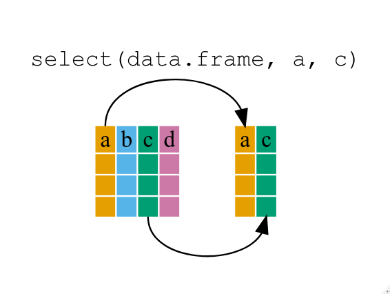Diagram illustrating use of select function to select two columns of a data frame If we want to remove one column only from the gapminder data, for example, removing the continent column.

R

smaller_gapminder_data <- select(gapminder, -continent)

If we open up year_country_gdp we’ll see that it only contains the year, country and gdpPercap. Above we used ‘normal’ grammar, but the strengths of dplyr lie in combining several functions using pipes. Since the pipes grammar is unlike anything we’ve seen in R before, let’s repeat what we’ve done above using pipes.

R

year_country_gdp <- gapminder %>% select(year, country, gdpPercap)

To help you understand why we wrote that in that way, let’s walk through it step by step. First we summon the gapminder data frame and pass it on, using the pipe symbol %>%, to the next step, which is the select() function. In this case we don’t specify which data object we use in the select() function since in gets that from the previous pipe. Fun Fact: There is a good chance you have encountered pipes before in the shell. In R, a pipe symbol is %>% while in the shell it is | but the concept is the same!

Tip: Renaming data frame columns in dplyr

In Chapter 4 we covered how you can rename columns with base R by assigning a value to the output of the names() function. Just like select, this is a bit cumbersome, but thankfully dplyr has a rename() function.

Within a pipeline, the syntax is rename(new_name = old_name). For example, we may want to rename the gdpPercap column name from our select() statement above.

R

tidy_gdp <- year_country_gdp %>% rename(gdp_per_capita = gdpPercap)

head(tidy_gdp)

OUTPUT

  year     country gdp_per_capita
1 1952 Afghanistan       779.4453
2 1957 Afghanistan       820.8530
3 1962 Afghanistan       853.1007
4 1967 Afghanistan       836.1971
5 1972 Afghanistan       739.9811
6 1977 Afghanistan       786.1134

Using filter()

If we now want to move forward with the above, but only with European countries, we can combine select and filter

R

year_country_gdp_euro <- gapminder %>%
    filter(continent == "Europe") %>%
    select(year, country, gdpPercap)

If we now want to show life expectancy of European countries but only for a specific year (e.g., 2007), we can do as below.

R

europe_lifeExp_2007 <- gapminder %>%
  filter(continent == "Europe", year == 2007) %>%
  select(country, lifeExp)

Challenge 1

Write a single command (which can span multiple lines and includes pipes) that will produce a data frame that has the African values for lifeExp, country and year, but not for other Continents. How many rows does your data frame have and why?

Solution to Challenge 1

R

year_country_lifeExp_Africa <- gapminder %>%
                           filter(continent == "Africa") %>%
                           select(year, country, lifeExp)

As with last time, first we pass the gapminder data frame to the filter() function, then we pass the filtered version of the gapminder data frame to the select() function. Note: The order of operations is very important in this case. If we used ‘select’ first, filter would not be able to find the variable continent since we would have removed it in the previous step.

Using group_by()

Now, we were supposed to be reducing the error prone repetitiveness of what can be done with base R, but up to now we haven’t done that since we would have to repeat the above for each continent. Instead of filter(), which will only pass observations that meet your criteria (in the above: continent=="Europe"), we can use group_by(), which will essentially use every unique criteria that you could have used in filter.

R

str(gapminder)

OUTPUT

'data.frame':	1704 obs. of  6 variables:
 $ country  : chr  "Afghanistan" "Afghanistan" "Afghanistan" "Afghanistan" ...
 $ year     : int  1952 1957 1962 1967 1972 1977 1982 1987 1992 1997 ...
 $ pop      : num  8425333 9240934 10267083 11537966 13079460 ...
 $ continent: chr  "Asia" "Asia" "Asia" "Asia" ...
 $ lifeExp  : num  28.8 30.3 32 34 36.1 ...
 $ gdpPercap: num  779 821 853 836 740 ...

R

str(gapminder %>% group_by(continent))

OUTPUT

gropd_df [1,704 × 6] (S3: grouped_df/tbl_df/tbl/data.frame)
 $ country  : chr [1:1704] "Afghanistan" "Afghanistan" "Afghanistan" "Afghanistan" ...
 $ year     : int [1:1704] 1952 1957 1962 1967 1972 1977 1982 1987 1992 1997 ...
 $ pop      : num [1:1704] 8425333 9240934 10267083 11537966 13079460 ...
 $ continent: chr [1:1704] "Asia" "Asia" "Asia" "Asia" ...
 $ lifeExp  : num [1:1704] 28.8 30.3 32 34 36.1 ...
 $ gdpPercap: num [1:1704] 779 821 853 836 740 ...
 - attr(*, "groups")= tibble [5 × 2] (S3: tbl_df/tbl/data.frame)
  ..$ continent: chr [1:5] "Africa" "Americas" "Asia" "Europe" ...
  ..$ .rows    : list<int> [1:5]
  .. ..$ : int [1:624] 25 26 27 28 29 30 31 32 33 34 ...
  .. ..$ : int [1:300] 49 50 51 52 53 54 55 56 57 58 ...
  .. ..$ : int [1:396] 1 2 3 4 5 6 7 8 9 10 ...
  .. ..$ : int [1:360] 13 14 15 16 17 18 19 20 21 22 ...
  .. ..$ : int [1:24] 61 62 63 64 65 66 67 68 69 70 ...
  .. ..@ ptype: int(0)
  ..- attr(*, ".drop")= logi TRUE

You will notice that the structure of the data frame where we used group_by() (grouped_df) is not the same as the original gapminder (data.frame). A grouped_df can be thought of as a list where each item in the listis a data.frame which contains only the rows that correspond to the a particular value continent (at least in the example above).

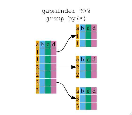
Diagram illustrating how the group by function oraganizes a data frame into groups

Using summarize()

The above was a bit on the uneventful side but group_by() is much more exciting in conjunction with summarize(). This will allow us to create new variable(s) by using functions that repeat for each of the continent-specific data frames. That is to say, using the group_by() function, we split our original data frame into multiple pieces, then we can run functions (e.g. mean() or sd()) within summarize().

R

gdp_bycontinents <- gapminder %>%
    group_by(continent) %>%
    summarize(mean_gdpPercap = mean(gdpPercap))

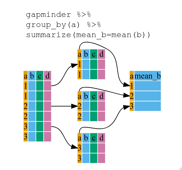
Diagram illustrating the use of group by and summarize together to create a new variable

R

continent mean_gdpPercap
     <fctr>          <dbl>
1    Africa       2193.755
2  Americas       7136.110
3      Asia       7902.150
4    Europe      14469.476
5   Oceania      18621.609

That allowed us to calculate the mean gdpPercap for each continent, but it gets even better.

Challenge 2

Calculate the average life expectancy per country. Which has the longest average life expectancy and which has the shortest average life expectancy?

Solution to Challenge 2

R

lifeExp_bycountry <- gapminder %>%
   group_by(country) %>%
   summarize(mean_lifeExp = mean(lifeExp))
lifeExp_bycountry %>%
   filter(mean_lifeExp == min(mean_lifeExp) | mean_lifeExp == max(mean_lifeExp))

OUTPUT

# A tibble: 2 × 2
  country      mean_lifeExp
  <chr>               <dbl>
1 Iceland              76.5
2 Sierra Leone         36.8

Another way to do this is to use the dplyr function arrange(), which arranges the rows in a data frame according to the order of one or more variables from the data frame. It has similar syntax to other functions from the dplyr package. You can use desc() inside arrange() to sort in descending order.

R

lifeExp_bycountry %>%
   arrange(mean_lifeExp) %>%
   head(1)

OUTPUT

# A tibble: 1 × 2
  country      mean_lifeExp
  <chr>               <dbl>
1 Sierra Leone         36.8

R

lifeExp_bycountry %>%
   arrange(desc(mean_lifeExp)) %>%
   head(1)

OUTPUT

# A tibble: 1 × 2
  country mean_lifeExp
  <chr>          <dbl>
1 Iceland         76.5

Alphabetical order works too

R

lifeExp_bycountry %>%
   arrange(desc(country)) %>%
   head(1)

OUTPUT

# A tibble: 1 × 2
  country  mean_lifeExp
  <chr>           <dbl>
1 Zimbabwe         52.7

The function group_by() allows us to group by multiple variables. Let’s group by year and continent.

R

gdp_bycontinents_byyear <- gapminder %>%
    group_by(continent, year) %>%
    summarize(mean_gdpPercap = mean(gdpPercap))

OUTPUT

`summarise()` has grouped output by 'continent'. You can override using the
`.groups` argument.

That is already quite powerful, but it gets even better! You’re not limited to defining 1 new variable in summarize().

R

gdp_pop_bycontinents_byyear <- gapminder %>%
    group_by(continent, year) %>%
    summarize(mean_gdpPercap = mean(gdpPercap),
              sd_gdpPercap = sd(gdpPercap),
              mean_pop = mean(pop),
              sd_pop = sd(pop))

OUTPUT

`summarise()` has grouped output by 'continent'. You can override using the
`.groups` argument.

count() and n()

A very common operation is to count the number of observations for each group. The dplyr package comes with two related functions that help with this.

For instance, if we wanted to check the number of countries included in the dataset for the year 2002, we can use the count() function. It takes the name of one or more columns that contain the groups we are interested in, and we can optionally sort the results in descending order by adding sort=TRUE:

R

gapminder %>%
    filter(year == 2002) %>%
    count(continent, sort = TRUE)

OUTPUT

  continent  n
1    Africa 52
2      Asia 33
3    Europe 30
4  Americas 25
5   Oceania  2

If we need to use the number of observations in calculations, the n() function is useful. It will return the total number of observations in the current group rather than counting the number of observations in each group within a specific column. For instance, if we wanted to get the standard error of the life expectency per continent:

R

gapminder %>%
    group_by(continent) %>%
    summarize(se_le = sd(lifeExp)/sqrt(n()))

OUTPUT

# A tibble: 5 × 2
  continent se_le
  <chr>     <dbl>
1 Africa    0.366
2 Americas  0.540
3 Asia      0.596
4 Europe    0.286
5 Oceania   0.775

You can also chain together several summary operations; in this case calculating the minimum, maximum, mean and se of each continent’s per-country life-expectancy:

R

gapminder %>%
    group_by(continent) %>%
    summarize(
      mean_le = mean(lifeExp),
      min_le = min(lifeExp),
      max_le = max(lifeExp),
      se_le = sd(lifeExp)/sqrt(n()))

OUTPUT

# A tibble: 5 × 5
  continent mean_le min_le max_le se_le
  <chr>       <dbl>  <dbl>  <dbl> <dbl>
1 Africa       48.9   23.6   76.4 0.366
2 Americas     64.7   37.6   80.7 0.540
3 Asia         60.1   28.8   82.6 0.596
4 Europe       71.9   43.6   81.8 0.286
5 Oceania      74.3   69.1   81.2 0.775

Using mutate()

We can also create new variables prior to (or even after) summarizing information using mutate().

R

gdp_pop_bycontinents_byyear <- gapminder %>%
    mutate(gdp_billion = gdpPercap*pop/10^9) %>%
    group_by(continent,year) %>%
    summarize(mean_gdpPercap = mean(gdpPercap),
              sd_gdpPercap = sd(gdpPercap),
              mean_pop = mean(pop),
              sd_pop = sd(pop),
              mean_gdp_billion = mean(gdp_billion),
              sd_gdp_billion = sd(gdp_billion))

OUTPUT

`summarise()` has grouped output by 'continent'. You can override using the
`.groups` argument.

Connect mutate with logical filtering: ifelse

When creating new variables, we can hook this with a logical condition. A simple combination of mutate() and ifelse() facilitates filtering right where it is needed: in the moment of creating something new. This easy-to-read statement is a fast and powerful way of discarding certain data (even though the overall dimension of the data frame will not change) or for updating values depending on this given condition.

R

## keeping all data but "filtering" after a certain condition
# calculate GDP only for people with a life expectation above 25
gdp_pop_bycontinents_byyear_above25 <- gapminder %>%
    mutate(gdp_billion = ifelse(lifeExp > 25, gdpPercap * pop / 10^9, NA)) %>%
    group_by(continent, year) %>%
    summarize(mean_gdpPercap = mean(gdpPercap),
              sd_gdpPercap = sd(gdpPercap),
              mean_pop = mean(pop),
              sd_pop = sd(pop),
              mean_gdp_billion = mean(gdp_billion),
              sd_gdp_billion = sd(gdp_billion))

OUTPUT

`summarise()` has grouped output by 'continent'. You can override using the
`.groups` argument.

R

## updating only if certain condition is fullfilled
# for life expectations above 40 years, the gpd to be expected in the future is scaled
gdp_future_bycontinents_byyear_high_lifeExp <- gapminder %>%
    mutate(gdp_futureExpectation = ifelse(lifeExp > 40, gdpPercap * 1.5, gdpPercap)) %>%
    group_by(continent, year) %>%
    summarize(mean_gdpPercap = mean(gdpPercap),
              mean_gdpPercap_expected = mean(gdp_futureExpectation))

OUTPUT

`summarise()` has grouped output by 'continent'. You can override using the
`.groups` argument.

Combining `dplyr` and `ggplot2`

First install and load ggplot2:

R

install.packages('ggplot2')

R

library("ggplot2")

In the plotting lesson we looked at how to make a multi-panel figure by adding a layer of facet panels using ggplot2. Here is the code we used (with some extra comments):

R

# Filter countries located in the Americas
americas <- gapminder[gapminder$continent == "Americas", ]
# Make the plot
ggplot(data = americas, mapping = aes(x = year, y = lifeExp)) +
  geom_line() +
  facet_wrap( ~ country) +
  theme(axis.text.x = element_text(angle = 45))

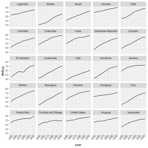
This code makes the right plot but it also creates an intermediate variable (americas) that we might not have any other uses for. Just as we used %>% to pipe data along a chain of dplyr functions we can use it to pass data to ggplot(). Because %>% replaces the first argument in a function we don’t need to specify the data = argument in the ggplot() function. By combining dplyr and ggplot2 functions we can make the same figure without creating any new variables or modifying the data.

R

gapminder %>%
  # Filter countries located in the Americas
  filter(continent == "Americas") %>%
  # Make the plot
  ggplot(mapping = aes(x = year, y = lifeExp)) +
  geom_line() +
  facet_wrap( ~ country) +
  theme(axis.text.x = element_text(angle = 45))

More examples of using the function mutate() and the ggplot2 package.

R

gapminder %>%
  # extract first letter of country name into new column
  mutate(startsWith = substr(country, 1, 1)) %>%
  # only keep countries starting with A or Z
  filter(startsWith %in% c("A", "Z")) %>%
  # plot lifeExp into facets
  ggplot(aes(x = year, y = lifeExp, colour = continent)) +
  geom_line() +
  facet_wrap(vars(country)) +
  theme_minimal()

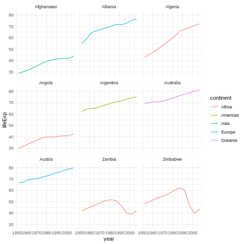
Advanced Challenge

Calculate the average life expectancy in 2002 of 2 randomly selected countries for each continent. Then arrange the continent names in reverse order. Hint: Use the dplyr functions arrange() and sample_n(), they have similar syntax to other dplyr functions.

Solution to Advanced Challenge

R

lifeExp_2countries_bycontinents <- gapminder %>%
   filter(year==2002) %>%
   group_by(continent) %>%
   sample_n(2) %>%
   summarize(mean_lifeExp=mean(lifeExp)) %>%
   arrange(desc(mean_lifeExp))

Other great resources

R for Data Science (online book)
Data Wrangling Cheat sheet (pdf file)
Introduction to dplyr (online documentation)
Data wrangling with R and RStudio (online video)
Tidyverse Skills for Data Science (online book)

Key Points

Use the dplyr package to manipulate data frames.
Use select() to choose variables from a data frame.
Use filter() to choose data based on values.
Use group_by() and summarize() to work with subsets of data.
Use mutate() to create new variables.

Content from Data Frame Manipulation with tidyr

Last updated on 2025-07-01 | Edit this page

Estimated time: 45 minutes

Overview

Questions

How can I change the layout of a data frame?

Objectives

To understand the concepts of ‘longer’ and ‘wider’ data frame formats and be able to convert between them with tidyr.

Researchers often want to reshape their data frames from ‘wide’ to ‘longer’ layouts, or vice-versa. The ‘long’ layout or format is where:

each column is a variable
each row is an observation

In the purely ‘long’ (or ‘longest’) format, you usually have 1 column for the observed variable and the other columns are ID variables.

For the ‘wide’ format each row is often a site/subject/patient and you have multiple observation variables containing the same type of data. These can be either repeated observations over time, or observation of multiple variables (or a mix of both). You may find data input may be simpler or some other applications may prefer the ‘wide’ format. However, many of R‘s functions have been designed assuming you have ’longer’ formatted data. This tutorial will help you efficiently transform your data shape regardless of original format.

Diagram illustrating the difference between a wide versus long layout of a data frame

Long and wide data frame layouts mainly affect readability. For humans, the wide format is often more intuitive since we can often see more of the data on the screen due to its shape. However, the long format is more machine readable and is closer to the formatting of databases. The ID variables in our data frames are similar to the fields in a database and observed variables are like the database values.

Getting started

First install the packages if you haven’t already done so (you probably installed dplyr in the previous lesson):

R

#install.packages("tidyr")
#install.packages("dplyr")

Load the packages

R

library("tidyr")
library("dplyr")

First, lets look at the structure of our original gapminder data frame:

R

str(gapminder)

OUTPUT

'data.frame':	1704 obs. of  6 variables:
 $ country  : chr  "Afghanistan" "Afghanistan" "Afghanistan" "Afghanistan" ...
 $ year     : int  1952 1957 1962 1967 1972 1977 1982 1987 1992 1997 ...
 $ pop      : num  8425333 9240934 10267083 11537966 13079460 ...
 $ continent: chr  "Asia" "Asia" "Asia" "Asia" ...
 $ lifeExp  : num  28.8 30.3 32 34 36.1 ...
 $ gdpPercap: num  779 821 853 836 740 ...

Challenge 1

Is gapminder a purely long, purely wide, or some intermediate format?

Solution to Challenge 1

The original gapminder data.frame is in an intermediate format. It is not purely long since it had multiple observation variables (pop,lifeExp,gdpPercap).

Sometimes, as with the gapminder dataset, we have multiple types of observed data. It is somewhere in between the purely ‘long’ and ‘wide’ data formats. We have 3 “ID variables” (continent, country, year) and 3 “Observation variables” (pop,lifeExp,gdpPercap). This intermediate format can be preferred despite not having ALL observations in 1 column given that all 3 observation variables have different units. There are few operations that would need us to make this data frame any longer (i.e. 4 ID variables and 1 Observation variable).

While using many of the functions in R, which are often vector based, you usually do not want to do mathematical operations on values with different units. For example, using the purely long format, a single mean for all of the values of population, life expectancy, and GDP would not be meaningful since it would return the mean of values with 3 incompatible units. The solution is that we first manipulate the data either by grouping (see the lesson on dplyr), or we change the structure of the data frame. Note: Some plotting functions in R actually work better in the wide format data.

From wide to long format with pivot_longer()

Until now, we’ve been using the nicely formatted original gapminder dataset, but ‘real’ data (i.e. our own research data) will never be so well organized. Here let’s start with the wide formatted version of the gapminder dataset.

Download the wide version of the gapminder data from this link to a csv file and save it in your data folder.

We’ll load the data file and look at it. Note: we don’t want our continent and country columns to be factors, so we use the stringsAsFactors argument for read.csv() to disable that.

R

gap_wide <- read.csv("data/gapminder_wide.csv", stringsAsFactors = FALSE)
str(gap_wide)

OUTPUT

'data.frame':	142 obs. of  38 variables:
 $ continent     : chr  "Africa" "Africa" "Africa" "Africa" ...
 $ country       : chr  "Algeria" "Angola" "Benin" "Botswana" ...
 $ gdpPercap_1952: num  2449 3521 1063 851 543 ...
 $ gdpPercap_1957: num  3014 3828 960 918 617 ...
 $ gdpPercap_1962: num  2551 4269 949 984 723 ...
 $ gdpPercap_1967: num  3247 5523 1036 1215 795 ...
 $ gdpPercap_1972: num  4183 5473 1086 2264 855 ...
 $ gdpPercap_1977: num  4910 3009 1029 3215 743 ...
 $ gdpPercap_1982: num  5745 2757 1278 4551 807 ...
 $ gdpPercap_1987: num  5681 2430 1226 6206 912 ...
 $ gdpPercap_1992: num  5023 2628 1191 7954 932 ...
 $ gdpPercap_1997: num  4797 2277 1233 8647 946 ...
 $ gdpPercap_2002: num  5288 2773 1373 11004 1038 ...
 $ gdpPercap_2007: num  6223 4797 1441 12570 1217 ...
 $ lifeExp_1952  : num  43.1 30 38.2 47.6 32 ...
 $ lifeExp_1957  : num  45.7 32 40.4 49.6 34.9 ...
 $ lifeExp_1962  : num  48.3 34 42.6 51.5 37.8 ...
 $ lifeExp_1967  : num  51.4 36 44.9 53.3 40.7 ...
 $ lifeExp_1972  : num  54.5 37.9 47 56 43.6 ...
 $ lifeExp_1977  : num  58 39.5 49.2 59.3 46.1 ...
 $ lifeExp_1982  : num  61.4 39.9 50.9 61.5 48.1 ...
 $ lifeExp_1987  : num  65.8 39.9 52.3 63.6 49.6 ...
 $ lifeExp_1992  : num  67.7 40.6 53.9 62.7 50.3 ...
 $ lifeExp_1997  : num  69.2 41 54.8 52.6 50.3 ...
 $ lifeExp_2002  : num  71 41 54.4 46.6 50.6 ...
 $ lifeExp_2007  : num  72.3 42.7 56.7 50.7 52.3 ...
 $ pop_1952      : num  9279525 4232095 1738315 442308 4469979 ...
 $ pop_1957      : num  10270856 4561361 1925173 474639 4713416 ...
 $ pop_1962      : num  11000948 4826015 2151895 512764 4919632 ...
 $ pop_1967      : num  12760499 5247469 2427334 553541 5127935 ...
 $ pop_1972      : num  14760787 5894858 2761407 619351 5433886 ...
 $ pop_1977      : num  17152804 6162675 3168267 781472 5889574 ...
 $ pop_1982      : num  20033753 7016384 3641603 970347 6634596 ...
 $ pop_1987      : num  23254956 7874230 4243788 1151184 7586551 ...
 $ pop_1992      : num  26298373 8735988 4981671 1342614 8878303 ...
 $ pop_1997      : num  29072015 9875024 6066080 1536536 10352843 ...
 $ pop_2002      : int  31287142 10866106 7026113 1630347 12251209 7021078 15929988 4048013 8835739 614382 ...
 $ pop_2007      : int  33333216 12420476 8078314 1639131 14326203 8390505 17696293 4369038 10238807 710960 ...

Diagram illustrating the wide format of the gapminder data frame

To change this very wide data frame layout back to our nice, intermediate (or longer) layout, we will use one of the two available pivot functions from the tidyr package. To convert from wide to a longer format, we will use the pivot_longer() function. pivot_longer() makes datasets longer by increasing the number of rows and decreasing the number of columns, or ‘lengthening’ your observation variables into a single variable.

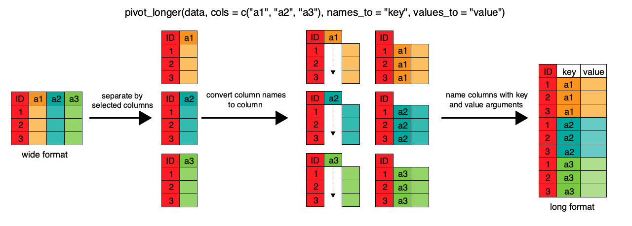
Diagram illustrating how pivot longer reorganizes a data frame from a wide to long format

R

gap_long <- gap_wide %>%
  pivot_longer(
    cols = c(starts_with('pop'), starts_with('lifeExp'), starts_with('gdpPercap')),
    names_to = "obstype_year", values_to = "obs_values"
  )
str(gap_long)

OUTPUT

tibble [5,112 × 4] (S3: tbl_df/tbl/data.frame)
 $ continent   : chr [1:5112] "Africa" "Africa" "Africa" "Africa" ...
 $ country     : chr [1:5112] "Algeria" "Algeria" "Algeria" "Algeria" ...
 $ obstype_year: chr [1:5112] "pop_1952" "pop_1957" "pop_1962" "pop_1967" ...
 $ obs_values  : num [1:5112] 9279525 10270856 11000948 12760499 14760787 ...

Here we have used piping syntax which is similar to what we were doing in the previous lesson with dplyr. In fact, these are compatible and you can use a mix of tidyr and dplyr functions by piping them together.

We first provide to pivot_longer() a vector of column names that will be pivoted into longer format. We could type out all the observation variables, but as in the select() function (see dplyr lesson), we can use the starts_with() argument to select all variables that start with the desired character string. pivot_longer() also allows the alternative syntax of using the - symbol to identify which variables are not to be pivoted (i.e. ID variables).

The next arguments to pivot_longer() are names_to for naming the column that will contain the new ID variable (obstype_year) and values_to for naming the new amalgamated observation variable (obs_value). We supply these new column names as strings.

Diagram illustrating the long format of the gapminder data

R

gap_long <- gap_wide %>%
  pivot_longer(
    cols = c(-continent, -country),
    names_to = "obstype_year", values_to = "obs_values"
  )
str(gap_long)

OUTPUT

tibble [5,112 × 4] (S3: tbl_df/tbl/data.frame)
 $ continent   : chr [1:5112] "Africa" "Africa" "Africa" "Africa" ...
 $ country     : chr [1:5112] "Algeria" "Algeria" "Algeria" "Algeria" ...
 $ obstype_year: chr [1:5112] "gdpPercap_1952" "gdpPercap_1957" "gdpPercap_1962" "gdpPercap_1967" ...
 $ obs_values  : num [1:5112] 2449 3014 2551 3247 4183 ...

That may seem trivial with this particular data frame, but sometimes you have 1 ID variable and 40 observation variables with irregular variable names. The flexibility is a huge time saver!

Now obstype_year actually contains 2 pieces of information, the observation type (pop,lifeExp, or gdpPercap) and the year. We can use the separate() function to split the character strings into multiple variables

R

gap_long <- gap_long %>% separate(obstype_year, into = c('obs_type', 'year'), sep = "_")
gap_long$year <- as.integer(gap_long$year)

Challenge 2

Using gap_long, calculate the mean life expectancy, population, and gdpPercap for each continent. Hint: use the group_by() and summarize() functions we learned in the dplyr lesson

Solution to Challenge 2

R

gap_long %>% group_by(continent, obs_type) %>%
   summarize(means=mean(obs_values))

OUTPUT

`summarise()` has grouped output by 'continent'. You can override using the
`.groups` argument.

OUTPUT

# A tibble: 15 × 3
# Groups:   continent [5]
   continent obs_type       means
   <chr>     <chr>          <dbl>
 1 Africa    gdpPercap     2194.
 2 Africa    lifeExp         48.9
 3 Africa    pop        9916003.
 4 Americas  gdpPercap     7136.
 5 Americas  lifeExp         64.7
 6 Americas  pop       24504795.
 7 Asia      gdpPercap     7902.
 8 Asia      lifeExp         60.1
 9 Asia      pop       77038722.
10 Europe    gdpPercap    14469.
11 Europe    lifeExp         71.9
12 Europe    pop       17169765.
13 Oceania   gdpPercap    18622.
14 Oceania   lifeExp         74.3
15 Oceania   pop        8874672.

From long to intermediate format with pivot_wider()

It is always good to check work. So, let’s use the second pivot function, pivot_wider(), to ‘widen’ our observation variables back out. pivot_wider() is the opposite of pivot_longer(), making a dataset wider by increasing the number of columns and decreasing the number of rows. We can use pivot_wider() to pivot or reshape our gap_long to the original intermediate format or the widest format. Let’s start with the intermediate format.

The pivot_wider() function takes names_from and values_from arguments.

To names_from we supply the column name whose contents will be pivoted into new output columns in the widened data frame. The corresponding values will be added from the column named in the values_from argument.

R

gap_normal <- gap_long %>%
  pivot_wider(names_from = obs_type, values_from = obs_values)
dim(gap_normal)

OUTPUT

[1] 1704    6

R

dim(gapminder)

OUTPUT

[1] 1704    6

R

names(gap_normal)

OUTPUT

[1] "continent" "country"   "year"      "gdpPercap" "lifeExp"   "pop"

R

names(gapminder)

OUTPUT

[1] "country"   "year"      "pop"       "continent" "lifeExp"   "gdpPercap"

Now we’ve got an intermediate data frame gap_normal with the same dimensions as the original gapminder, but the order of the variables is different. Let’s fix that before checking if they are all.equal().

R

gap_normal <- gap_normal[, names(gapminder)]
all.equal(gap_normal, gapminder)

OUTPUT

[1] "Attributes: < Component \"class\": Lengths (3, 1) differ (string compare on first 1) >"
[2] "Attributes: < Component \"class\": 1 string mismatch >"
[3] "Component \"country\": 1704 string mismatches"
[4] "Component \"pop\": Mean relative difference: 1.634504"
[5] "Component \"continent\": 1212 string mismatches"
[6] "Component \"lifeExp\": Mean relative difference: 0.203822"
[7] "Component \"gdpPercap\": Mean relative difference: 1.162302"

R

head(gap_normal)

OUTPUT

# A tibble: 6 × 6
  country  year      pop continent lifeExp gdpPercap
  <chr>   <int>    <dbl> <chr>       <dbl>     <dbl>
1 Algeria  1952  9279525 Africa       43.1     2449.
2 Algeria  1957 10270856 Africa       45.7     3014.
3 Algeria  1962 11000948 Africa       48.3     2551.
4 Algeria  1967 12760499 Africa       51.4     3247.
5 Algeria  1972 14760787 Africa       54.5     4183.
6 Algeria  1977 17152804 Africa       58.0     4910.

R

head(gapminder)

OUTPUT

      country year      pop continent lifeExp gdpPercap
1 Afghanistan 1952  8425333      Asia  28.801  779.4453
2 Afghanistan 1957  9240934      Asia  30.332  820.8530
3 Afghanistan 1962 10267083      Asia  31.997  853.1007
4 Afghanistan 1967 11537966      Asia  34.020  836.1971
5 Afghanistan 1972 13079460      Asia  36.088  739.9811
6 Afghanistan 1977 14880372      Asia  38.438  786.1134

We’re almost there, the original was sorted by country, then year.

R

gap_normal <- gap_normal %>% arrange(country, year)
all.equal(gap_normal, gapminder)

OUTPUT

[1] "Attributes: < Component \"class\": Lengths (3, 1) differ (string compare on first 1) >"
[2] "Attributes: < Component \"class\": 1 string mismatch >"

That’s great! We’ve gone from the longest format back to the intermediate and we didn’t introduce any errors in our code.

Now let’s convert the long all the way back to the wide. In the wide format, we will keep country and continent as ID variables and pivot the observations across the 3 metrics (pop,lifeExp,gdpPercap) and time (year). First we need to create appropriate labels for all our new variables (time*metric combinations) and we also need to unify our ID variables to simplify the process of defining gap_wide.

R

gap_temp <- gap_long %>% unite(var_ID, continent, country, sep = "_")
str(gap_temp)

OUTPUT

tibble [5,112 × 4] (S3: tbl_df/tbl/data.frame)
 $ var_ID    : chr [1:5112] "Africa_Algeria" "Africa_Algeria" "Africa_Algeria" "Africa_Algeria" ...
 $ obs_type  : chr [1:5112] "gdpPercap" "gdpPercap" "gdpPercap" "gdpPercap" ...
 $ year      : int [1:5112] 1952 1957 1962 1967 1972 1977 1982 1987 1992 1997 ...
 $ obs_values: num [1:5112] 2449 3014 2551 3247 4183 ...

R

gap_temp <- gap_long %>%
    unite(ID_var, continent, country, sep = "_") %>%
    unite(var_names, obs_type, year, sep = "_")
str(gap_temp)

OUTPUT

tibble [5,112 × 3] (S3: tbl_df/tbl/data.frame)
 $ ID_var    : chr [1:5112] "Africa_Algeria" "Africa_Algeria" "Africa_Algeria" "Africa_Algeria" ...
 $ var_names : chr [1:5112] "gdpPercap_1952" "gdpPercap_1957" "gdpPercap_1962" "gdpPercap_1967" ...
 $ obs_values: num [1:5112] 2449 3014 2551 3247 4183 ...

Using unite() we now have a single ID variable which is a combination of continent,country,and we have defined variable names. We’re now ready to pipe in pivot_wider()

R

gap_wide_new <- gap_long %>%
  unite(ID_var, continent, country, sep = "_") %>%
  unite(var_names, obs_type, year, sep = "_") %>%
  pivot_wider(names_from = var_names, values_from = obs_values)
str(gap_wide_new)

OUTPUT

tibble [142 × 37] (S3: tbl_df/tbl/data.frame)
 $ ID_var        : chr [1:142] "Africa_Algeria" "Africa_Angola" "Africa_Benin" "Africa_Botswana" ...
 $ gdpPercap_1952: num [1:142] 2449 3521 1063 851 543 ...
 $ gdpPercap_1957: num [1:142] 3014 3828 960 918 617 ...
 $ gdpPercap_1962: num [1:142] 2551 4269 949 984 723 ...
 $ gdpPercap_1967: num [1:142] 3247 5523 1036 1215 795 ...
 $ gdpPercap_1972: num [1:142] 4183 5473 1086 2264 855 ...
 $ gdpPercap_1977: num [1:142] 4910 3009 1029 3215 743 ...
 $ gdpPercap_1982: num [1:142] 5745 2757 1278 4551 807 ...
 $ gdpPercap_1987: num [1:142] 5681 2430 1226 6206 912 ...
 $ gdpPercap_1992: num [1:142] 5023 2628 1191 7954 932 ...
 $ gdpPercap_1997: num [1:142] 4797 2277 1233 8647 946 ...
 $ gdpPercap_2002: num [1:142] 5288 2773 1373 11004 1038 ...
 $ gdpPercap_2007: num [1:142] 6223 4797 1441 12570 1217 ...
 $ lifeExp_1952  : num [1:142] 43.1 30 38.2 47.6 32 ...
 $ lifeExp_1957  : num [1:142] 45.7 32 40.4 49.6 34.9 ...
 $ lifeExp_1962  : num [1:142] 48.3 34 42.6 51.5 37.8 ...
 $ lifeExp_1967  : num [1:142] 51.4 36 44.9 53.3 40.7 ...
 $ lifeExp_1972  : num [1:142] 54.5 37.9 47 56 43.6 ...
 $ lifeExp_1977  : num [1:142] 58 39.5 49.2 59.3 46.1 ...
 $ lifeExp_1982  : num [1:142] 61.4 39.9 50.9 61.5 48.1 ...
 $ lifeExp_1987  : num [1:142] 65.8 39.9 52.3 63.6 49.6 ...
 $ lifeExp_1992  : num [1:142] 67.7 40.6 53.9 62.7 50.3 ...
 $ lifeExp_1997  : num [1:142] 69.2 41 54.8 52.6 50.3 ...
 $ lifeExp_2002  : num [1:142] 71 41 54.4 46.6 50.6 ...
 $ lifeExp_2007  : num [1:142] 72.3 42.7 56.7 50.7 52.3 ...
 $ pop_1952      : num [1:142] 9279525 4232095 1738315 442308 4469979 ...
 $ pop_1957      : num [1:142] 10270856 4561361 1925173 474639 4713416 ...
 $ pop_1962      : num [1:142] 11000948 4826015 2151895 512764 4919632 ...
 $ pop_1967      : num [1:142] 12760499 5247469 2427334 553541 5127935 ...
 $ pop_1972      : num [1:142] 14760787 5894858 2761407 619351 5433886 ...
 $ pop_1977      : num [1:142] 17152804 6162675 3168267 781472 5889574 ...
 $ pop_1982      : num [1:142] 20033753 7016384 3641603 970347 6634596 ...
 $ pop_1987      : num [1:142] 23254956 7874230 4243788 1151184 7586551 ...
 $ pop_1992      : num [1:142] 26298373 8735988 4981671 1342614 8878303 ...
 $ pop_1997      : num [1:142] 29072015 9875024 6066080 1536536 10352843 ...
 $ pop_2002      : num [1:142] 31287142 10866106 7026113 1630347 12251209 ...
 $ pop_2007      : num [1:142] 33333216 12420476 8078314 1639131 14326203 ...

Challenge 3

Take this 1 step further and create a gap_ludicrously_wide format data by pivoting over countries, year and the 3 metrics? Hint this new data frame should only have 5 rows.

Solution to Challenge 3

R

gap_ludicrously_wide <- gap_long %>%
   unite(var_names, obs_type, year, country, sep = "_") %>%
   pivot_wider(names_from = var_names, values_from = obs_values)

Now we have a great ‘wide’ format data frame, but the ID_var could be more usable, let’s separate it into 2 variables with separate()

R

gap_wide_betterID <- separate(gap_wide_new, ID_var, c("continent", "country"), sep="_")
gap_wide_betterID <- gap_long %>%
    unite(ID_var, continent, country, sep = "_") %>%
    unite(var_names, obs_type, year, sep = "_") %>%
    pivot_wider(names_from = var_names, values_from = obs_values) %>%
    separate(ID_var, c("continent","country"), sep = "_")
str(gap_wide_betterID)

OUTPUT

tibble [142 × 38] (S3: tbl_df/tbl/data.frame)
 $ continent     : chr [1:142] "Africa" "Africa" "Africa" "Africa" ...
 $ country       : chr [1:142] "Algeria" "Angola" "Benin" "Botswana" ...
 $ gdpPercap_1952: num [1:142] 2449 3521 1063 851 543 ...
 $ gdpPercap_1957: num [1:142] 3014 3828 960 918 617 ...
 $ gdpPercap_1962: num [1:142] 2551 4269 949 984 723 ...
 $ gdpPercap_1967: num [1:142] 3247 5523 1036 1215 795 ...
 $ gdpPercap_1972: num [1:142] 4183 5473 1086 2264 855 ...
 $ gdpPercap_1977: num [1:142] 4910 3009 1029 3215 743 ...
 $ gdpPercap_1982: num [1:142] 5745 2757 1278 4551 807 ...
 $ gdpPercap_1987: num [1:142] 5681 2430 1226 6206 912 ...
 $ gdpPercap_1992: num [1:142] 5023 2628 1191 7954 932 ...
 $ gdpPercap_1997: num [1:142] 4797 2277 1233 8647 946 ...
 $ gdpPercap_2002: num [1:142] 5288 2773 1373 11004 1038 ...
 $ gdpPercap_2007: num [1:142] 6223 4797 1441 12570 1217 ...
 $ lifeExp_1952  : num [1:142] 43.1 30 38.2 47.6 32 ...
 $ lifeExp_1957  : num [1:142] 45.7 32 40.4 49.6 34.9 ...
 $ lifeExp_1962  : num [1:142] 48.3 34 42.6 51.5 37.8 ...
 $ lifeExp_1967  : num [1:142] 51.4 36 44.9 53.3 40.7 ...
 $ lifeExp_1972  : num [1:142] 54.5 37.9 47 56 43.6 ...
 $ lifeExp_1977  : num [1:142] 58 39.5 49.2 59.3 46.1 ...
 $ lifeExp_1982  : num [1:142] 61.4 39.9 50.9 61.5 48.1 ...
 $ lifeExp_1987  : num [1:142] 65.8 39.9 52.3 63.6 49.6 ...
 $ lifeExp_1992  : num [1:142] 67.7 40.6 53.9 62.7 50.3 ...
 $ lifeExp_1997  : num [1:142] 69.2 41 54.8 52.6 50.3 ...
 $ lifeExp_2002  : num [1:142] 71 41 54.4 46.6 50.6 ...
 $ lifeExp_2007  : num [1:142] 72.3 42.7 56.7 50.7 52.3 ...
 $ pop_1952      : num [1:142] 9279525 4232095 1738315 442308 4469979 ...
 $ pop_1957      : num [1:142] 10270856 4561361 1925173 474639 4713416 ...
 $ pop_1962      : num [1:142] 11000948 4826015 2151895 512764 4919632 ...
 $ pop_1967      : num [1:142] 12760499 5247469 2427334 553541 5127935 ...
 $ pop_1972      : num [1:142] 14760787 5894858 2761407 619351 5433886 ...
 $ pop_1977      : num [1:142] 17152804 6162675 3168267 781472 5889574 ...
 $ pop_1982      : num [1:142] 20033753 7016384 3641603 970347 6634596 ...
 $ pop_1987      : num [1:142] 23254956 7874230 4243788 1151184 7586551 ...
 $ pop_1992      : num [1:142] 26298373 8735988 4981671 1342614 8878303 ...
 $ pop_1997      : num [1:142] 29072015 9875024 6066080 1536536 10352843 ...
 $ pop_2002      : num [1:142] 31287142 10866106 7026113 1630347 12251209 ...
 $ pop_2007      : num [1:142] 33333216 12420476 8078314 1639131 14326203 ...

R

all.equal(gap_wide, gap_wide_betterID)

OUTPUT

[1] "Attributes: < Component \"class\": Lengths (1, 3) differ (string compare on first 1) >"
[2] "Attributes: < Component \"class\": 1 string mismatch >"

There and back again!

Other great resources

R for Data Science (online book)
Data Wrangling Cheat sheet (pdf file)
Introduction to tidyr (online documentation)
Data wrangling with R and RStudio (online video)

Key Points

Use the tidyr package to change the layout of data frames.
Use pivot_longer() to go from wide to longer layout.
Use pivot_wider() to go from long to wider layout.

Content from Producing Reports With knitr

Last updated on 2025-07-01 | Edit this page

Estimated time: 75 minutes

Overview

Questions

How can I integrate software and reports?

Objectives

Understand the value of writing reproducible reports
Learn how to recognise and compile the basic components of an R Markdown file
Become familiar with R code chunks, and understand their purpose, structure and options
Demonstrate the use of inline chunks for weaving R outputs into text blocks, for example when discussing the results of some calculations
Be aware of alternative output formats to which an R Markdown file can be exported

Data analysis reports

Data analysts tend to write a lot of reports, describing their analyses and results, for their collaborators or to document their work for future reference.

Many new users begin by first writing a single R script containing all of their work, and then share the analysis by emailing the script and various graphs as attachments. But this can be cumbersome, requiring a lengthy discussion to explain which attachment was which result.

Writing formal reports with Word or LaTeX can simplify this process by incorporating both the analysis report and output graphs into a single document. But tweaking formatting to make figures look correct and fixing obnoxious page breaks can be tedious and lead to a lengthy “whack-a-mole” game of fixing new mistakes resulting from a single formatting change.

Creating a report as a web page (which is an html file) using R Markdown makes things easier. The report can be one long stream, so tall figures that wouldn’t ordinarily fit on one page can be kept at full size and easier to read, since the reader can simply keep scrolling. Additionally, the formatting of and R Markdown document is simple and easy to modify, allowing you to spend more time on your analyses instead of writing reports.

Literate programming

Ideally, such analysis reports are reproducible documents: If an error is discovered, or if some additional subjects are added to the data, you can just re-compile the report and get the new or corrected results rather than having to reconstruct figures, paste them into a Word document, and hand-edit various detailed results.

The key R package here is knitr. It allows you to create a document that is a mixture of text and chunks of code. When the document is processed by knitr, chunks of code will be executed, and graphs or other results will be inserted into the final document.

This sort of idea has been called “literate programming”.

knitr allows you to mix basically any type of text with code from different programming languages, but we recommend that you use R Markdown, which mixes Markdown with R. Markdown is a light-weight mark-up language for creating web pages.

Creating an R Markdown file

Within RStudio, click File → New File → R Markdown and you’ll get a dialog box like this:

Screenshot of the New R Markdown file dialogue box in RStudio

You can stick with the default (HTML output), but give it a title.

Basic components of R Markdown

The initial chunk of text (header) contains instructions for R to specify what kind of document will be created, and the options chosen. You can use the header to give your document a title, author, date, and tell it what type of output you want to produce. In this case, we’re creating an html document.

---
title: "Initial R Markdown document"
author: "Karl Broman"
date: "April 23, 2015"
output: html_document
---

You can delete any of those fields if you don’t want them included. The double-quotes aren’t strictly necessary in this case. They’re mostly needed if you want to include a colon in the title.

RStudio creates the document with some example text to get you started. Note below that there are chunks like

```{r}
summary(cars)
```

These are chunks of R code that will be executed by knitr and replaced by their results. More on this later.

Markdown

Markdown is a system for writing web pages by marking up the text much as you would in an email rather than writing html code. The marked-up text gets converted to html, replacing the marks with the proper html code.

For now, let’s delete all of the stuff that’s there and write a bit of markdown.

You make things bold using two asterisks, like this: **bold**, and you make things italics by using underscores, like this: _italics_.

You can make a bulleted list by writing a list with hyphens or asterisks with a space between the list and other text, like this:

A list:

* bold with double-asterisks
* italics with underscores
* code-type font with backticks

or like this:

A second list:

- bold with double-asterisks
- italics with underscores
- code-type font with backticks

Each will appear as:

bold with double-asterisks
italics with underscores
code-type font with backticks

You can use whatever method you prefer, but be consistent. This maintains the readability of your code.

You can make a numbered list by just using numbers. You can even use the same number over and over if you want:

1. bold with double-asterisks
1. italics with underscores
1. code-type font with backticks

This will appear as:

bold with double-asterisks
italics with underscores
code-type font with backticks

You can make section headers of different sizes by initiating a line with some number of # symbols:

# Title
## Main section
### Sub-section
#### Sub-sub section

You compile the R Markdown document to an html webpage by clicking the “Knit” button in the upper-left.

Challenge 1

Create a new R Markdown document. Delete all of the R code chunks and write a bit of Markdown (some sections, some italicized text, and an itemized list).

Convert the document to a webpage.

Solution to Challenge 1

In RStudio, select File > New file > R Markdown…

Delete the placeholder text and add the following:

# Introduction

## Background on Data

This report uses the *gapminder* dataset, which has columns that include:

* country
* continent
* year
* lifeExp
* pop
* gdpPercap

## Background on Methods

Then click the ‘Knit’ button on the toolbar to generate an html document (webpage).

A bit more Markdown

You can make a hyperlink like this: [Carpentries Home Page](https://carpentries.org/).

You can include an image file like this: ![The Carpentries Logo](https://carpentries.org/assets/img/TheCarpentries.svg)

You can do subscripts (e.g., F₂) with F~2~ and superscripts (e.g., F²) with F^2^.

If you know how to write equations in LaTeX, you can use $ $ and $$ $$ to insert math equations, like $E = mc^2$ and

$$y = \mu + \sum_{i=1}^p \beta_i x_i + \epsilon$$

You can review Markdown syntax by navigating to the “Markdown Quick Reference” under the “Help” field in the toolbar at the top of RStudio.

R code chunks

The real power of Markdown comes from mixing markdown with chunks of code. This is R Markdown. When processed, the R code will be executed; if they produce figures, the figures will be inserted in the final document.

The main code chunks look like this:

```{r load_data} gapminder

That is, you place a chunk of R code between ```{r chunk_name} and ```. You should give each chunk a unique name, as they will help you to fix errors and, if any graphs are produced, the file names are based on the name of the code chunk that produced them. You can create code chunks quickly in RStudio using the shortcuts Ctrl+Alt+I on Windows and Linux, or Cmd+Option+I on Mac.

Challenge 2

Add code chunks to:

Load the ggplot2 package
Read the gapminder data
Create a plot

Solution to Challenge 2

```{r load-ggplot2}
library("ggplot2")
```

```{r read-gapminder-data}
gapminder
```{r make-plot}
plot(lifeExp ~ year, data = gapminder)
```

How things get compiled

When you press the “Knit” button, the R Markdown document is processed by knitr and a plain Markdown document is produced (as well as, potentially, a set of figure files): the R code is executed and replaced by both the input and the output; if figures are produced, links to those figures are included.

The Markdown and figure documents are then processed by the tool pandoc, which converts the Markdown file into an html file, with the figures embedded.

Chunk options

There are a variety of options to affect how the code chunks are treated. Here are some examples:

Use echo=FALSE to avoid having the code itself shown.
Use results="hide" to avoid having any results printed.
Use eval=FALSE to have the code shown but not evaluated.
Use warning=FALSE and message=FALSE to hide any warnings or messages produced.
Use fig.height and fig.width to control the size of the figures produced (in inches).

So you might write:

```{r load_libraries, echo=FALSE, message=FALSE}
library("dplyr")
library("ggplot2")
```

Often there will be particular options that you’ll want to use repeatedly; for this, you can set global chunk options, like so:

```{r global_options, echo=FALSE}
knitr::opts_chunk$set(fig.path="Figs/", message=FALSE, warning=FALSE,
                      echo=FALSE, results="hide", fig.width=11)
```

The fig.path option defines where the figures will be saved. The / here is really important; without it, the figures would be saved in the standard place but just with names that begin with Figs.

If you have multiple R Markdown files in a common directory, you might want to use fig.path to define separate prefixes for the figure file names, like fig.path="Figs/cleaning-" and fig.path="Figs/analysis-".

Challenge 3

Use chunk options to control the size of a figure and to hide the code.

Solution to Challenge 3

```{r echo = FALSE, fig.width = 3}
plot(faithful)
```

You can review all of the R chunk options by navigating to the “R Markdown Cheat Sheet” under the “Cheatsheets” section of the “Help” field in the toolbar at the top of RStudio.

Inline R code

You can make every number in your report reproducible. Use `r and ` for an in-line code chunk, like so: `r round(some_value, 2)`. The code will be executed and replaced with the value of the result.

Don’t let these in-line chunks get split across lines.

Perhaps precede the paragraph with a larger code chunk that does calculations and defines variables, with include=FALSE for that larger chunk (which is the same as echo=FALSE and results="hide").

Rounding can produce differences in output in such situations. You may want 2.0, but round(2.03, 1) will give just 2.

The myround function in the R/broman package handles this.

Challenge 4

Try out a bit of in-line R code.

Solution to Challenge 4

Here’s some inline code to determine that 2 + 2 = 4.

Other output options

You can also convert R Markdown to a PDF or a Word document. Click the little triangle next to the “Knit” button to get a drop-down menu. Or you could put pdf_document or word_document in the initial header of the file.

Tip: Creating PDF documents

Creating .pdf documents may require installation of some extra software. The R package tinytex provides some tools to help make this process easier for R users. With tinytex installed, run tinytex::install_tinytex() to install the required software (you’ll only need to do this once) and then when you knit to pdf tinytex will automatically detect and install any additional LaTeX packages that are needed to produce the pdf document. Visit the tinytex website for more information.

Tip: Visual markdown editing in RStudio

RStudio versions 1.4 and later include visual markdown editing mode. In visual editing mode, markdown expressions (like **bold words**) are transformed to the formatted appearance (bold words) as you type. This mode also includes a toolbar at the top with basic formatting buttons, similar to what you might see in common word processing software programs. You can turn visual editing on and off by pressing the Icon for turning on and off the visual editing mode in RStudio, which looks like a pair of compasses button in the top right corner of your R Markdown document.

Resources

Knitr in a knutshell tutorial
Dynamic Documents with R and knitr (book)
R Markdown documentation
R Markdown cheat sheet
Getting started with R Markdown
R Markdown: The Definitive Guide (book by Rstudio team)
Reproducible Reporting
The Ecosystem of R Markdown
Introducing Bookdown

Key Points

Mix reporting written in R Markdown with software written in R.
Specify chunk options to control formatting.
Use knitr to convert these documents into PDF and other formats.

Content from Writing Good Software

Last updated on 2025-07-01 | Edit this page

Estimated time: 15 minutes

Overview

Questions

How can I write software that other people can use?

Objectives

Describe best practices for writing R and explain the justification for each.

Structure your project folder

Keep your project folder structured, organized and tidy, by creating subfolders for your code files, manuals, data, binaries, output plots, etc. It can be done completely manually, or with the help of RStudio’s New Project functionality, or a designated package, such as ProjectTemplate.

Tip: ProjectTemplate - a possible solution

One way to automate the management of projects is to install the third-party package, ProjectTemplate. This package will set up an ideal directory structure for project management. This is very useful as it enables you to have your analysis pipeline/workflow organised and structured. Together with the default RStudio project functionality and Git you will be able to keep track of your work as well as be able to share your work with collaborators.

Install ProjectTemplate.
Load the library
Initialise the project:

R

install.packages("ProjectTemplate")
library("ProjectTemplate")
create.project("../my_project_2", merge.strategy = "allow.non.conflict")

For more information on ProjectTemplate and its functionality visit the home page ProjectTemplate

Make code readable

The most important part of writing code is making it readable and understandable. You want someone else to be able to pick up your code and be able to understand what it does: more often than not this someone will be you 6 months down the line, who will otherwise be cursing past-self.

Documentation: tell us what and why, not how

When you first start out, your comments will often describe what a command does, since you’re still learning yourself and it can help to clarify concepts and remind you later. However, these comments aren’t particularly useful later on when you don’t remember what problem your code is trying to solve. Try to also include comments that tell you why you’re solving a problem, and what problem that is. The how can come after that: it’s an implementation detail you ideally shouldn’t have to worry about.

Keep your code modular

Our recommendation is that you should separate your functions from your analysis scripts, and store them in a separate file that you source when you open the R session in your project. This approach is nice because it leaves you with an uncluttered analysis script, and a repository of useful functions that can be loaded into any analysis script in your project. It also lets you group related functions together easily.

Break down problem into bite size pieces

When you first start out, problem solving and function writing can be daunting tasks, and hard to separate from code inexperience. Try to break down your problem into digestible chunks and worry about the implementation details later: keep breaking down the problem into smaller and smaller functions until you reach a point where you can code a solution, and build back up from there.

Know that your code is doing the right thing

Make sure to test your functions!

Don’t repeat yourself

Functions enable easy reuse within a project. If you see blocks of similar lines of code through your project, those are usually candidates for being moved into functions.

If your calculations are performed through a series of functions, then the project becomes more modular and easier to change. This is especially the case for which a particular input always gives a particular output.

Remember to be stylish

Apply consistent style to your code.

Key Points

Keep your project folder structured, organized and tidy.
Document what and why, not how.
Break programs into short single-purpose functions.
Write re-runnable tests.
Don’t repeat yourself.
Be consistent in naming, indentation, and other aspects of style.